Effect of Record Length on Prediction of Extreme Events Using River Flow Data

item and our policy information available from the repository home page for further information.

Author(s):Hames, Dominic

Article title: Effect of Record Length on Prediction of Extreme Events Using River Flow Data

Year of publication:2006

Citation: Hames, D. (2006) ‘Effect of Record Length on Prediction of Extreme Events Using River Flow Data’Proceedings of the AC&T, pp.107-112.

Link to published version:

EFFECT OF RECORD LENGTH ON PREDICTION OF

EXTREME EVENTS USING RIVER FLOW DATA

Dominic Hames

Built Environment Research Group

[email protected]

Abstract: This paper considers the effect of record length on the sensitivity of extreme predictions

based on the analysis of annually recorded maximum flow records for a number of locations worldwide. Locations have been chosen based on the criterion of a minimum of 100 years of standardised records, with extremes that closely follow standard statistical techniques.

Based on the analysis carried out, confidence of extreme predictions appear to be a function of the log of the return period event required, the reciprocal of the square root of the record length and a parameter unique for each river. Using the techniques outlined in this paper, methods are proposed to give confidence on extreme predictions using limited data sets. However, more work is required to define the unique parameter for each river, which has not been considered in this paper.

1. Introduction

The determination of extreme events for design purposes is based on the analysis of past records. With often little data available, predictions can become highly variable with an unknown level of confidence. As with time more data becomes available, predictions usually become more robust and can indicate extreme predictions noticeably different from previous estimates. The effect of unreliable predictions can result in increased costs due to over designed schemes, or continuing damage and often wasted design costs due to under designed schemes.

This paper investigates the effect of record length on the sensitivity of extreme predictions of river flow using standardised annual maxima records at locations around the world where at least 100 years of records are available. Locations chosen were based on records published in Herschy, 2003 and 2004. Locations which were observed to not follow the well known Gumbel distribution were excluded from the analysis. This gave data sets where predictions of extremes using the full record

length could be considered robust, and where sub-samples of data sets would follow an underlying statistical distribution. Based on the criteria outlined above, 9 locations were analysed which are outlined in Table 1.

2. Analysis methodology

position (Marriott et al, 2004) as this is the distribution followed by a Monte Carlo simulation. The distribution of the return period estimates was investigated as the variation of the predictions relative to the return periods determined using the original (standardised) annual maxima record.

2.1. Extreme predictions

The Gumbel distribution is given by equation 1.

( )

F exp (1)

where:

ξ is the position parameter

θ is the scale parameter This can be written as:

ξ θ

η = X + (2)

where:

( )

(

)

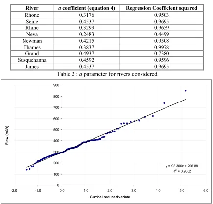
Using the Gumbel distribution in this form, the values of ξ and θ can be determined by a least squares analysis and this is shown for the River Thames data using the binomial plotting position in Figure 1.

2.2. Distribution of simulated extremes

Based on the analysis carried out, extreme estimates of flow from simulated annual maxima were seen to follow a normal distribution of near mean zero, and standard deviations proportional to the reciprocal of the square root of the simulation. This is shown for 20 year simulations for the River Thames in Figure 2, where the difference (Ef) is given by equation 3.

C C S f E η η η −

= (3)

where:

ηC is the calculated ‘actual’ flow

ηS is the estimated flow from the simulation

Considering different simulation lengths, the standard deviation of Ef was found to be

approximated by equation 4.

( )

σ (4)

where:

σT is the standard deviation of Ef

T is the return period required

n is the record length

a is a constant (different for each river)

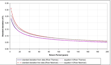
This is shown for the River Thames and the River Newman in Figure 3. This shows good correlation, particularly for the River Thames. The correlation for the River Newman is typical of the remaining rivers considered in this paper (apart from the River Neva which is quite poor).

The values of a appear to be unique for each individual river, and for the rivers considered in this paper are shown in Table 2. Also shown in this table are estimates of the regression coefficient squared, which gives an idea of the accuracy of the fit of equation 4.

3. Accuracy of extreme estimates

( )

 

± =

n T a z

a

C S

ln 1 _%

η

η (5)

where:

z% is the standard normal variable

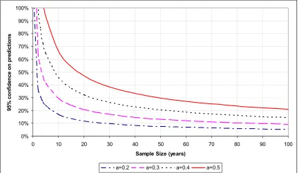
Considering the 95% confidence in predictions, this is shown for different values of a for a 100 year return period event in Figure 4. For the River Thames (for example), which has an estimated a

value of 0.3837, the 100 year return period event would be estimated to be calculated (for 95% confidence) to within 43% using a 10 year record length, and within 19% using a 50 year record length.

4. Conclusions

Based on the analysis in this paper, confidence in estimates of extremes from limited data sets for the rivers considered has been proposed. However, for these rivers large data sets are already available and predictions can be considered robust. For rivers with limited data sets (less than about 20 years), predictions are less robust and the methods proposed in this paper can be used to investigate the confidence in predictions of extremes.

Two problems clearly exist in using this technique in these cases. These are the determination of the a parameter in equation 4 for the level of accuracy, and the ‘actual’ flow (ηC) for use in equation 5. Although

the variation in the a parameter for limited data sets has not been studied in this paper, this could easily be considered in a future publication. This would give a level of confidence in its prediction, and confidence placed on its value. The variation of the ‘actual’ flow could also be investigated however, as this is the variable that confidence is being placed on, an

investigation of this type could be considered spurious and is not necessary.

5. References

Gumbel E.J, Statistics of Extremes, Columbia University Press, New York, 1958.

Herschy R, World Catalogue of Maximum Observed Floods, IAHS Publication 284, IAHS Press, 2003.

Herschy R, World Catalogue of Maximum Observed Floods (Errata and Supplementary Data), IAHS Press, 2004.

River Gauging Location Catchment Range Years

Rhone Beaucaire (France) 96500 km2 1845 - 1982 138

Seine Paris (France) 44300 km2 _{1733 - 1982 245}

Rhine Lobith (Holland) 160000 km2 _{1901 - 2000 100}

Neva Novosaratovka (Russia) 281000 km2 _{1859 - 1979 118}

Newman Smalininkai (Russia) 81200 km2 1812 - 1978 164

Thames Kingston (UK) 9948 km2 _{1884 - 2003 120}

Grand Lansing (USA) 3190 km2 _{1901 - 2000 100}

Susquehanna Harrisburg (USA) 62400 km2 _{1891 - 2001 111}

James Buchanan (USA) 5374 km2 _{1893 - 1999 107}

Table 1: Locations and records considered

River a coefficient (equation 4) Regression Coefficient squared

Rhone 0.3176 0.9503

Seine 0.4537 0.9695

Rhine 0.3299 0.9659

Neva 0.2483 0.4499

Newman 0.4215 0.9508

Thames 0.3837 0.9978

Grand 0.4937 0.7380

Susquehanna 0.4592 0.9596

James 0.4537 0.9695

Table 2 : a parameter for rivers considered

Figure 1 : Extreme estimates of flow for the River Thames (for 2003) y = 92.306x + 296.88

R2 _{= 0.9852}

0 100 200 300 400 500 600 700 800 900

-2.0 -1.0 0.0 1.0 2.0 3.0 4.0 5.0 6.0

Gumbel reduced variate

Fl

o

w

(

m

3/

Figure 2 : Error in estimates for 20 year simulations (River Thames)

Figure 3 : Variation in standard deviation of Ef for different return periods

0.0 0.5 1.0 1.5 2.0 2.5 3.0 3.5 4.0

-0.4 -0.3 -0.2 -0.1 0.0 0.1 0.2 0.3 0.4

Ef

E

f

de

ns

it

y

10 year return period 50 year return period

0.00 0.05 0.10 0.15 0.20 0.25 0.30 0.35

0 20 40 60 80 100 120 140 160 180 200

Return Period (years)

S

ta

nda

rd

de

vi

at

io

n of E

f

Figure 4 : 95% confidence in predictions for different a values (100 year return period event)

0% 10% 20% 30% 40% 50% 60% 70% 80% 90% 100%

0 10 20 30 40 50 60 70 80 90 100

Sample Size (years)

95

%

c

onf

ide

n

ce

on pr

ed

ic

ti

ons