Efficient Identification of Linchpin Vertices in Dependence Clusters

Efficient Identification of Linchpin Vertices in Dependence Clusters

David Binkley, Loyola University Maryland Nicolas Gold, University College London Mark Harman, University College London Syed Islam, University College London Jens Krinke, University College London

Zheng Li, Beijing University of Chemical Technology

Several authors have found evidence of large dependence clusters in the source code of a diverse range of systems, domains, and programming languages. This raises the question of how we might efficiently locate the fragments of code that give rise to large dependence clusters. We introduce an algorithm for the identification oflinchpinvertices, which hold together large dependence clusters, and prove correctness properties for the algorithm’s primary innovations. We also report the results of an empirical study concerning the reduction in analysis time that our algorithm yields over its predecessor using a collection of 38 programs containing almost half a million lines of code. Our empirical findings indicate improvements of almost two orders of magnitude, making it possible to process larger programs for which it would have previously been impractical.

Categories and Subject Descriptors: D.2.5 [Software Engineering]: Testing and Debugging—debugging aids; D.2.6 [ Soft-ware Engineering]: Programming Environments; E.1 [Data Structures]: Graphs; F.3.2 [Logics and Meanings of Pro-grams]: Semantics of Programming Languages—Program analysis

General Terms: Algorithms, Performance

Additional Key Words and Phrases: Slicing, Internal Representation, Performance Enhancement, Empirical Study

1. INTRODUCTION

in isolation and therefore difficult to take any action to ameliorate their potentially harmful effects without major restructuring. This motivated the study oflinchpinedges and vertices [Binkley and Harman 2009]. A linchpin is a single edge or vertex in a program’s dependence graph through which so much dependence flows that the linchpin holds together a large cluster.

One obvious and natural way to identify a linchpin is to remove it, re-construct the dependence graph, and then compare the ‘before’ and ‘after’ graphs to see if the large dependence cluster has either disappeared or reduced in size. This na¨ıve approach was implemented as a proof of concept to demonstrate that such linchpins do indeed exist [Binkley and Harman 2009]. That is, therearesingle vertices and edges in real world systems, the removal of which causes large dependence clusters to essentially disappear.

This na¨ıve algorithm is useful as a demonstration that linchpins exist, but it must consider all vertices as potential linchpins. Unfortunately, this limits its applicability as a useful research tool. That is, the computational resources required for even mid-sized programs are simply too great for the approach to be practical. In this paper we improve the applicability of the analysis from thousands of lines of code to tens of thousands of lines of code by developing a graph-pattern based theory that provides a foundation for more efficient linchpin detection. Finally, we introduce a new linchpin detection algorithm based on this theory and report on its performance with an empirical study of 38 programs containing a total of 494K lines of code.

The theory includes a ratio which we term the ‘risk ratio’. If the risk ratio is sufficiently small then we know that the impact (as captured by the ratio) of a set of vertices on large dependence clusters will be negligible. On this basis we are able to define a predicate that guards whether or not we are able to prune vertices from linchpin consideration. The theory establishes the required properties of the risk ratio, but only an empirical study can answer whether or not the guarding predicate that uses this ratio is satisfied sufficiently often to be useful for performance improvement. We therefore complement the theoretical study with an empirical study that investigates this question. We find that the predicate is satisfied in all but four of over a million cases. Furthermore, these four all occur with the strictest configuration in very small programs. This provides empirical evidence to support the claim that the theory is highly applicable in practice. Our empirical study also reports the performance improvement obtained by the new algorithm. Finally, we introduce and empirically study a tuning parameter (the search depth in what we call ‘fringe look ahead’). Our empirical study investigates the additional performance increase obtained using various values of the tuning parameter.

Using the new algorithm we were able to study several mid-sized programs ranging up to 66KLoC. This provides a relatively robust set of results on non-trivial systems upon which we draw evidence to support our empirical findings regarding the improved execution efficiency of the new algorithm. The results support our claim that the theoretical improvement of our algorithm is borne out in practice. For instance, to analyze the mid-sized programgo, which has 29,246 lines of code, using the na¨ıve approach takes 101 days. Using the tuned version of the new algorithm this time is reduced to just 8 days.

The primary contributions of the paper are as follows:

(1) Three theorems, proved in Section 3, identify situations in which it is possible to effectively exclude vertices from consideration as linchpins. These theoretical findings highlight opportu-nities for pruning the search for linchpins.

(2) Based on this theory, Section 4 introduces a more efficient linchpin search algorithm that ex-ploits the pruning opportunities to reduce search time. Section 4 also proves the algorithm’s correctness with respect to the theory introduced in Section 3.

vertex set reaching vertices(G,V,excluded edge kinds)

{

work list=V

answer=∅

whilework list! =∅

select and remove a vertexvfromwork list markv

insertvintoanswer

foreach unmarked vertexwsuch that there is an edgew→vwhose kind is not inexcluded edge kinds

insertwintowork list returnanswer

}

For SDGG,

b1(v)=reaching vertices(G,{v},{parameter-out})

b2(v)=reaching vertices(G,{v},{parameter-in, call})

Fig. 1. The functionreaching vertices[Binkley 1993] returns all vertices in SDGGfrom which there is a path to a vertex inV along edges whose edge-kind is something other than those in the setexcluded edge kinds.

the further performance improvements that can be obtained by tuning the basic algorithm.

2. BACKGROUND: LARGE DEPENDENCE CLUSTERS AND THEIR CAUSES

Dependence clusters can be defined in terms of program slices [Binkley and Harman 2005]. This section briefly reviews the definitions of slice, dependence clusters, and dependence cluster causes, to motivate the study of dependence clusters in general and of improved techniques for finding linchpins in particular. More detailed accounts can be found in the literature [Harman et al. 2009].

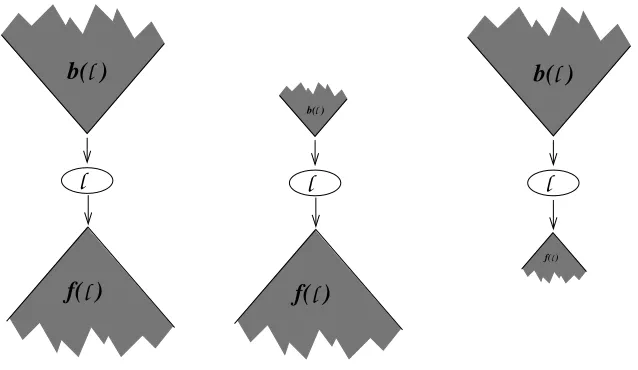
A backward slice identifies the parts of a program that potentially affect a selected computa-tion [Weiser 1984], while a forward slice identifies the parts of the program potentially affected by a selected computation [Horwitz et al. 1990; Reps and Yang 1988]. Both slices can be defined as the solution to graph reachability problems over a program’sSystem Dependence Graph(SDG) [Hor-witz et al. 1990] using two passes over the graph. The passes differ in their treatment of interproce-dural edges. For example, the backward slice taken with respect to SDG vertexv, denotedb(v), is computed by the first traversing only edges “up” into calling procedures while the second pass tra-verses only edges “down” into called procedures. Both passes exploit transitive dependence edges (summary edges) included at each call site to summarize the dependence paths through the called procedure. The two passes of a backward slice are referred to asb1andb2; thusb(v) =b2(b1(v)) where the slice taken with respect to a set of verticesV is defined as the union of the slices taken with respect to each vertexv ∈V. For a forward slicef(v) = f2(f1(v))wheref1traverses only edges “up” into calling procedures andf2traverses only edges “down” into called procedures.

Formalizing these slicing operators is done in terms of the interprocedural edges that enter and exit called procedures. Three such edge kinds exist in an SDG: aparameter-in edgerepresents the data dependence of a formal parameter on the value of the actual, aparameter-out edgerepresents the data dependence of an actual parameter on the final value of the formal as well as the data dependence from the returned value, and finally acall edge represents the control dependence of the called procedure on a call-site. Figure 1 provides the algorithm used to computeb1(v)andb2(v). The algorithm for forward slicing is the same except edges are traversed in the forward direction.

control

interprocedural data

summary

parameter−out call

parameter−in

call inc

x_in = a a = x_out

call inc call double

d_out = d double

d = d_in

d = d * 2 inc

x = x_in x_out = x

x = x + 1

Edge Key t = 42

x_in = t t = x_out d_in = t t = d_out

{ inc(x) double(d)

a = inc(a) { {

t = 42 x = x + 1 d = d * 2

t = inc(t) return x return d

t = double(t) } }

}

Fig. 2. An example SDG showing with slice taken with respect to the vertex labeledd = d * 2. The vertices of the slice are shown bold.

summarize paths through the called procedure, allow Pass 1 to include the initialization of t(t = 42) without descending into procedureinc. The second pass, which excludes parameter-in and call edges, starts from all the vertices encountered in the first pass. In particular, when starting from the vertex labeledx = x outthe slice descends into procedureincand thus includes the body of the procedure. Combined, the two passes respect calling context and thus correctly omit the first call on procedureinc. The vertices of the slice are shown in bold.

It is possible to compute the slice with respect to any SDG vertex. However, in the experiments only the vertices representing source code are considered as slice starting points. Furthermore, slice size is defined as the number of vertices representing source code encountered while slicing. Re-stricting attention to the vertices representing source code excludes several kinds of ‘internal’ ver-tices introduced by CodeSurfer [Grammatech Inc. 2002] (the tool used to build the SDGs). For example, an SDG includes pseudo-parameter vertices representing global variables potentially ac-cessed by a called procedure.

approximation has been empirically demonstrated to be over 99% accurate [Binkley and Harman 2005; Harman et al. 2009]. In the following definitions| · · · |is used to denote size. For a setS,|S|

denotes the number of elements inS, while for an SDGG, a sliceb(v), or an SDG pathP, size is the number of vertices that represent source code inG,b(v), or alongP, respectively, Using slice size, dependence clusters can be defined as follows

Definition1 (DEPENDENCECLUSTER).

Thedependence clusterfor vertexvof SDGGconsists of all vertices that have the same slice size asv:cluster(v) ={u∈G s.t.|b(u)|=|b(v)|}.2

Our previous work has demonstrated that large dependence clusters are surprisingly prevalent in traditional systems written in the C programming language, for both open and closed source systems [Harman et al. 2009; Binkley et al. 2008]. Other authors have subsequently replicated this finding in other languages and systems, both in open source and proprietary code [Besz´edes et al. 2007; Szegedi et al. 2007; Acharya and Robinson 2011]. Though our work has focused on C programs, large dependence clusters have also been found by other authors in C++ and Java systems [Besz´edes et al. 2007; Savernik 2007; Szegedi et al. 2007] and there is recent evidence that they are present in legacy Cobol systems [Hajnal and Forg´acs 2011].

Large dependence clusters have been linked to dependence ‘anti patterns’ or bad smells that reflect possible problems for on-going software maintenance and evolution [Savernik 2007; Binkley et al. 2008; Acharya and Robinson 2011]. Other authors have studied the relationship between faults, program size, and dependence clusters [Black et al. 2006], and between impact analysis and dependence clusters [Acharya and Robinson 2011; Harman et al. 2009]. The presence of large dependence clusters has also been suggested as an opportunity for refactoring intervention [Black et al. 2009; Binkley and Harman 2005; Islam et al. 2010a].

Because dependence clusters are believed to raise potential problems for software maintenance, testing, and comprehension, and because they have been shown to be highly prevalent in real sys-tems, a natural question arises: “What causes large dependence clusters?” Our previous work inves-tigated the global variables that contribute to creating large clusters of dependence [Binkley et al. 2009]. For example, the global variable representing the board in a chess program creates a large cluster involving all the pieces. Finding such a global variable can be important for understand-ing the causes of a cluster. However, global variables, by their nature, permeate the entire program scope and so the ability to take action based on this knowledge is limited. This motivates the study of linchpins: small localized pieces of code that cause (in the sense that they hold the cluster together) the formation of large dependence clusters.

The search for linchpins considers the impact of removing each potential linchpin on the de-pendence connections in the program. In an SDG the component whose removal has the smallest dependence impact is a single dependence edge. A vertex, which can have multiple incident edges, is the next smallest component. Because a linchpin edge’s target vertex must be a linchpin vertex, it is a quick process to identify linchpin edges once the linchpin vertices have been identified. This process simply considers each incoming edge of each linchpin vertex in turn [Binkley and Harman 2009]. Thus, in this paper, we characterize the answer to the question of what holds clusters together in terms of a search forlinchpin vertices.

Ignoring the dependencies of a linchpin vertex will cause the dependence cluster to disappear. For a vertex, it is sufficient to ignore either the vertex’s incomingoroutgoing dependence edges. Without loss of generality, the experiments ignore the incoming dependence edges.

40% 60% 80% 100%

0% 20%

0% 20% 40% 60% 80% 100%

40% 60% 80% 100%

0% 20%

0% 20% 40% 60% 80% 100%

40% 60% 80% 100%

0% 20%

0% 20% 40% 60% 80% 100%

MSG (a) – original MSG (b) – drop only MSG (c) – broken cluster

Fig. 3. The area under the MSG drops under two conditions: the slices of the cluster get smaller (center MSG), or when the cluster breaks (rightmost MSG). Thus, while a reduction in area is necessary, it is not a sufficient condition for cluster breaking.

paper use the percentage of the backward slices taken on thex-axis and the percentage of the entire program on they-axis.

In general the definitions laid out in the next section will work with an MSG constructed from any set of vertices. As mentioned above, for the empirical investigation presented in Section 5 the set of source-code representing vertices is used as both the slice starting points and when determining the size of a slice. Under this arrangement a cluster appears as a rectangle that is taller than it is wide.

The search considers changes in thearea under the MSG, denotedAMSG. This area is the sum

of all the slice sizes that make up the MSG. Formally, ifSCis the set of SDG vertices representing source code then

AMSG =

X

v∈SC

|b(v)|

As illustrated in Figure 3, areductionin area is a necessary but not a sufficient condition for iden-tifying alinchpinvertex. This is because there are two possible outcomes: adropand abreak. These two are illustrated by the center and right-most MSGs shown in Figure 3. Both show a reduction in area; however, the center MSG reflects only a reduction in the size of the backward slices that makeup up a cluster. Only the right-most MSG shows a true breaking of the cluster. These two are clear-cut extreme examples meant to illustrate the concepts of a drop and a break. In reality there are reductions that incorporate both effects. In the end, the decision if a reduction represents a drop or a break is subjective.

The detection algorithm presented in Section 4 reports all cases in which the reduction is greater than a threshold. These must then be inspected to determine if the area reduction represents a true breaking of a cluster. From the three example MSGs shown in Figure 3, it is clear that a reduction in area must accompany the breaking of a cluster, but does not imply the breaking of a cluster. Thus, to test if a Vertexl is a linchpin, the MSG for the program is constructed while ignoringl’s incoming dependence edges. If a significant reduction in area occurs, the resulting MSG can then be inspected to see if the cluster is broken.

x = 1

y = x + 1

z = x * y v

u 1

c

b a

l

Fig. 4. Simple Example of a vertex (highlighted in bold) that need not be considered as a potential linchpin.

3. THEORETICAL INVESTIGATION OF PROPERTIES OF DEPENDENCE CLUSTER CAUSES The na¨ıve linchpin search algorithm simply recomputes the MSG while ignoring the incoming de-pendence edges of each vertex in turn. MSG construction is computationally non-trivial and the inspection becomes tedious when considering programs with thousands of vertices. Thus, this sec-tion considers the efficient search for linchpin vertices. The search centers around several graph patterns that identify vertices thatcannotplay the role of a linchpin vertex. The section begins with two examples that illustrate the key concepts.

Figure 4 shows a Vertexl1 thatcannotbe a linchpin. This is because there are two paths con-necting Vertexv, labeledx = 1, to Vertexu, labeledz = x * y. Ignoringl1’s incoming dependence edges does not disconnectvanduand thus the level of ‘overall connectedness’ does not diminish. Consequently, a backward slice taken with respect to any vertex other thanl1(e.g.,aorb) continues to includevand the verticesvdepends on such asc; thus, the backward slice size of all slices except the one taken with respect tol1is unchanged.

Figure 5 shows a slightly more involved example in which one of the paths fromvtouincludes two verticesl1andl2(labeledt = x + 1andy = t + t). With this example, ignoring the incoming edges of Vertexl1changes only the sizes of the backward slices taken with respect tol1andl2, which have sizes one and two respectively when the incoming edges ofl1are ignored. Ignoring the incoming dependence edges ofl2has two effects. First, it reduces to one the size of the backward slice taken with respect tol2. Second, it reduces the size of all backward slices that includeuby one because they no longer includel1; however, these backward slices continue to includevand the vertices that it depends on such asc, thus, the reduction is small as formalized in the next section.

Building on these examples, three graph patterns are considered and then proven correct. Each pattern bounds the reduction in the area under the MSG,AMSG, that ignoring the incoming edges

of a potential linchpin vertex may have. This reduction is formalized by the following two small-impact properties. Both properties, as well as the remainder of the paper, include a parameter,κ, that denotes a minimum percentage area reduction below which ignoring a vertex’s incoming edges is deemed to have an insignificant impact onAMSG. The selection ofκis subjective. In the empirical

analysis of the next section, a range of values is considered.

When identifying vertices that have a small impact it is often useful to exclude from consideration the impact of a certain (small) set of vertices,V, on the area under the MSG, denotedAMSG\V.

x = 1

z = x * y t = x + 1

y = t + t

v

u 2

1

c

b a

l

l

Fig. 5. A more complex example involving a path of two vertices. Again the bold vertices need not be considered as potential linchpins.

except those vertices inV. Formally, ifSCis the set of vertices representing source code in an SDG then

AMSG\V =

X

v∈SC−V

|b(v)|

For example, in a graph where all vertices have exactly one edge targeting a common vertex, v, ignoringv’s incoming edges reduces the area under the MSG by almost 50%, but has no effect on the area underAMSG\{v}, which ignores the area attributed tov. Such a reduction never corresponds

to the breaking of a cluster and thus is uninteresting. The impact onAMSG\V andAMSG\∅(i.e.,

with and without ignoring any vertices) is formalized by the following two definitions:

Definition2 (STRONGSMALL-IMPACTPROPERTY).

Vertexvsatisfies thestrong small-impact propertyiff ignoring the incoming dependence edges ofv

can reduceAMSG(equivalentlyAMSG\∅) by at mostκpercent.

2

Definition3 (WEAKSMALL-IMPACTPROPERTY).

Given a (small) set for verticesV, Vertexvsatisfies theweak small-impact propertyiff ignoring the incoming dependence edges ofvcan reduce the area underAMSG\V by at mostκpercent.

2

A Vertexv that satisfies the strong small-impact property also satisfies the weak small-impact property, but not vice versa. Thus the strong version is preferred. Both are introduced because some-times the strong version cannot be proven to hold.

Definition4 (SAME-LEVELREALIZABLEPATH[REPS ANDROSAY1995]).

Let each call-site vertex in SDGGbe given a unique index from 1 tok. For each call siteci, label the outgoing parameter-in edges and the incoming parameter-out edges with the symbols “(i” and

“)i”, respectively; label the outgoing call edge with “(i”. A path inGis asame-level realizable

pathiff the sequence of symbols labeling the parameter-in, parameter-out, and call edges on the path is a string in the language of balanced parentheses generated from the nonterminal matched of the following grammar.

matched→matched(imatched)i for1≤i≤k

|

2

The formalization next describesvalid paths (Definition 5), the paths traversed while slicing: a vertexuinb(v)is connected to v by a valid path. In the general caseuandv are in different procedures called by a common ancestor. For example in Figure 2 ifuis the vertex labeledx = x + 1andvis the vertex labeledd = d * 2then the path fromutovis a valid path. A valid path includes two parts. The first connectsuto a vertex in the common ancestor (e.g., the vertex labeledt = x out), while the second connects this vertex tov. Valid paths and their two parts are used to formally define six slicing operators (Definition 6). Finally, a set of path composition rules is introduced.

Definition5 (VALIDPATH[REPS ANDROSAY1995]).

A path in SDGGis a (context) valid path iff the sequence of symbols labeling the parameter-in, parameter-out, and call edges on the path is a string in the language generated from nonterminal valid-path given by the following context-free grammar where the non-terminals b1f2-valid-path and b2f1-valid-path take their names from the two slicing passes used in the implementation of interprocedural slicing.

valid-path→b2f1-valid-path b1f2-valid-path

b2f1-valid-path

→b2f1-valid-path matched )i for1≤i≤k

|matched

b1f2-valid-path

→matched (ib1f2-valid-path for1≤i≤k

|matched

2

Example. For example, in Figure 2 there are two calls oninc, inc(a)and inc(t). In the SDG there are interprocedural parameter-in edges from each actual parameter to the vertex labeledx = x inthat represent the transfer of the actual to the formal. Symmetrically there are interprocedural parameter-out edges that represent the transfer of the returned value back to each caller. In terms of the grammar, the edges intoincare labeled(1and(2 while the edges back to the call sites are labeled)1and)2. Paths that match(1)1represent calls through the first call site,inc(a)and those that match(2)2represent calls through the second call site,inc(t). However any path that includes(1

)2is not a valid path as it represents enteringincfrom the first call site but returning to the second. One such path connects the vertex labeledx in = ato the vertex labeledd = d * 2

The interprocedural backward slice of an SDG taken with respect to Vertexv,b(v), includes the program components whose vertices are connected tovvia avalidpath. The interprocedural forward slice of an SDG taken with respect to Vertexv,f(v), includes the components whose vertices are reachable fromv via avalid path. Both slices are computed using two passes. This leads to the following six slicing operators for slicing SDGG.

b(v) ={u∈G|u→∗_{vis a valid path}}

b1(v) ={u∈G|u→∗_{vis ab}

1f2-valid path}

b2(v) ={u∈G|u→∗_{vis ab}

2f1-valid path}

f(v) ={u∈G|v→∗_{uis a valid path}}

f1(v) ={u∈G|v→∗_{uis ab}

2f1-valid path}

f2(v) ={u∈G|v→∗_{uis ab}

1f2-valid path}

2

Example. In Figure 2 let thev be the vertex labeledd = d * 2,ube the vertex labeledx = x + 1, andwbe the vertex labeledt = x out. In the SDG there is ab1f2-valid path fromwtovand a

b2f1-valid path fromutow. This placesw ∈ b1(v),u ∈ b2(w), andu ∈ b(v). Symmetrically,

w∈f1(u),v∈f2(w), andv∈f(u).

As noted before, the notation is overloaded such that each of the above slicing operators can be applied to a set of verticesV. The result is the union of the slices taken with respect to each vertex ofV. For example,b(V) =∪v∈Vb(v); thusf(v) =f2(f1(v))andb(v) =b2(b1(v)).

Finally, the search for linchpin vertices makes use of path composition, denotedp1◦p2, where pathp1’s final vertex is the same as pathp2’s first vertex. Some path compositions yield invalid paths. The following table describes the legal and illegal compositions.

Path Combinations

1 b1f2-valid path ◦ b1f2-valid path → b1f2-valid path 2 b1f2-valid path ◦ b2f1-valid path → invalid path 3 b1f2-valid path ◦ valid path → invalid path 4 b2f1-valid path ◦ b1f2-valid path → valid path 5 b2f1-valid path ◦ b2f1-valid path → b2f1-valid path 6 b2f1-valid path ◦ valid path → valid path 7 valid path ◦ b1f2-valid path → valid path 8 valid path ◦ b2f1-valid path → invalid path 9 valid path ◦ valid path → invalid path

Example. A valid path has two sections: the first (matchingb2f1-valid path) includes only un-matched)i’s, while the second (matchingb1f2-valid path) includes only unmatched(i’s. The first

composition rule notes that composing two paths with only unmatched(i’s leaves a path with only

unmatched(i’s. The second and third rules observe that the result of appending a path that includes

unmatched(i’s to a path that includes unmatched)i’s is not a valid path. For example, in Figure 2

composing the b1f2-valid path that connects the vertices labeledx in = aandx = x + 1with the

b2f1-valid path that connects the vertices labeledx = x + 1andt = x outresults in a path that enters

incthrough one call site but exists through the other; this path is not a valid path. However, as seen in the table, it is always legal to prefix a path with a path that contains unmatched)i’s (rules 4 and

6) and it is always legal to suffix a path with a path that contains unmatched(i’s (rules 4 and 7).

Building on these definitions, Theorem 1 identifies a condition in which the strong small-impact property holds.

Theorem1 (SMALLSLICE).

Letl be a vertex from SDGG. If|b(l)| ≤κAMSG/|G|or|f(l)| ≤κAMSG/|G|thenl satisfies the strong small-impact property.

f( )l l

b( )

l

f( )

l

l

l

b( )

l

l

f( )

l

b( )

Fig. 6. Illustration of the cases in Theorem 1. The worst-case illustrated on the left involves an SDG’s vertices being partitioned into three sets:{l},b(l), andf(l). The two cases of the proof are illustrated in the middle and on the right.

First, whenb(l)is small, the worst case area reduction is bounded by assuming that the vertices of b(l)are not reachable from any vertex other thanl (illustrated in the center of Figure 6). In this case, ignoring the incoming dependence edges ofl reduces each backward slice that includes

l by|b(l)|. In the worst casel is in every backward slice, which produces a maximal reduction of

|b(l)| × |G|. However, the assumption that|b(l)| ≤κAMSG/|G|implies that the total reduction is

at mostκAMSG and consequently the total area reduction is bound byκ.

Second, whenf(l)is small (illustrated in the right of Figure 6), note that the backward slices affected by ignoring the incoming edges ofl are those taken with respect to the vertices inf(l). Thus if|f(l)|is no more thanκAMSG/|G|then no more thanκAMSG/|G|backward slices are

affected. Because the maximal reduction for a slice is to be reduced to size zero (a reduction of at most|G|), the total area reduction is bounded by(κAMSG/|G|)× |G|, which is again bound byκ;

therefore, ifl has a small backward or a small forward slice then it satisfies the strong small-impact property.

As born out in the empirical investigation, the area reduction is often much smaller. For example it is unlikely thatl will be in every backward slice. Furthermore, the vertices ofb(l)often have connections to other parts of the SDG that do not go throughl. This is illustrated in the example shown in Figure 4 where ignoring the incoming edges ofl1doesnotremovevor its predecessors from backward slices that containu. Formalizing this observation is done in thedual-path property, which is built on top of the definition for valid paths (Definition 5). The dual-path property holds for two vertices when they are connected by two valid paths where one includes the selected vertex

l and the other does not.

Definition7 (DUAL-PATHPROPERTY).

Verticesl,v, andusatisfy theDual-Path Property, writtendpp(l, v, u), iff there are valid pathsvγu

andvβusuch thatl ∈γandl 6∈β.

2

v v = 4 call f(v)

f(a)

{ l b = a u u = a + b

c = f(42) x x = b + c return u

}

x u

l v

f

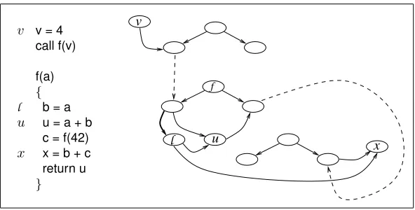
Fig. 7. An illustration of the the need fordpp2. Only a subgraph of the SDG is shown.

backward slice taken with respect tol1. This is because∀v∈b(l), dpp(l, v, u)and thus all backward slices that includel also includeuexcept the backward slice taken with respect tol. The value of the dual-path property is that this reduction can often be shown to be much smaller than|b(l1)|.

However, because interprocedural dependence is not transitive, an additional property is neces-sary. The issue arises when a backward slicesincludesl,u, and a vertexv0 wheredpp(l, v0, u), but the path fromv0_{touis ab1f2-valid path whileuis encountered during the second pass ofs.} In this case excluding verticesvfor whichdpp(l, v, u)overestimates the reduction (e.g., it errantly excludesv0).

Example. This situation is illustrated in Figure 7 where the sliceb(x)includes Vertices l,u, andv, and there are paths vγuandvβuwherel ∈ γ andl 6∈ β. Consider the situation when the incoming edge ofl (shown in bold) is ignored. During Pass 2 ofb(x)the slice descends intof

along the parameter-out edge through the recursive call (i.e.,c = f(42)). Becauseuis returned byf, the assignmentu = a + bis encountered while slicing; however, Pass 2 does not ascend to calling procedures and thus the slice does not ascend to the callf(v)and consequently does not reachv.

To correct for the over estimation, adppproperty is introduced to cover encounteringuduring a slice’s second pass:

Definition8 (SECONDPASSDUAL-PATHPROPERTY).

Verticesl,v, andusatisfy the second-pass Dual-Path Property, writtendpp2(l, v, u), iff there are two paths: valid pathvγuandb2f1-valid pathvβusuch thatl ∈γandl 6∈β.

2

Both dpp anddpp2 are used in the following theorem to prove that when certain dual paths exist,l satisfies the weak small-impact property (Definition 3). The weak version is used because the reduction for a backward slice taken with respect to certain vertices (e.g.,l) cannot be tightly bound. The first corollary to the theorem proves that under certain circumstances, the strong small-impact property also holds. For a vertex vin the slice b(x), the proof in essence splits the paths connectingvandxatl andu. The “top half” of these paths is captured by a dual-path property. while the “bottom half” is captured by the following vertex partitions based on a vertex’s backward slice’s inclusion of the two verticesl andu.

Set 1 - verticesxwherel 6∈b(x)

Set 2 - verticesxwherel ∈b(x)andu∈b(x)where there is a path fromutoxthat does not includel.

Example. These three sets can be illustrated using Figure 5 wherel is Vertexl1. In this example, Set 1 is{v, c}becauseb(v)andb(c)do not includel. For the remaining vertices (e.g., Vertexa)b(x)

includesl. Set 2 is{u, a, b}because the slice taken with respect to each of these vertices includes

u. Finally, Set 3 is{l2}becauseu,a, andbare not inb(l2)and whilec,v,l1, andl2are inb(l2), all paths connecting them tol2includel2.

Similar to the need for bothdppanddpp2, Set 2 is further partitioned based on the slicing pass in whichl anduare encountered.

Set 2.11 -l anduencountered during Pass 1

Set 2.12 -l encountered during Pass 1 anduduring Pass 2 (but not Pass 1) Set 2.21 -l encountered during Pass 2 (but not Pass 1) anduduring Pass 1 Set 2.22 -l anduencountered during Pass 2 (but not Pass 1)

Example.Verticesu,a, andbfrom Figure 5 are all in Set 2.11. Vertexxshown in Figure 7 is in Set 2.12 becausel is encountered during Pass 1 butuis not encountered until Pass 2.

Theorem2 (DUAL-PATHWEAKIMPACTTHEOREM).

Given an SDGGhavingV vertices, if there exists a Vertexusuch that for Set 2.11|b(l)− {v∈G|dpp(l, v, u)}| ≤κAMSG/V,

for Set 2.12|b(l)− {v∈G|dpp2(l, v, u)}| ≤κAMSG/V, for Set 2.21|b2(l)− {v∈G|dpp(l, v, u)}| ≤κAMSG/V, and

for Set 2.22|b2(l)− {v∈G|dpp2(l, v, u)}| ≤κAMSG/V

thenl satisfies the weak small-impact property. In particular, the area reduction underAMSG\Set 3 is bound byκ.

PROOF. The proof is a case analysis using the above partitions. For the first partition, Set 1, slices withoutl are unchanged when ignoringl’s incoming edges. Next consider Set 2.11, which includes slices wherel anduare encountered during Pass 1. Assume thatb(x)is such a slice. Thus there are b1f2-valid paths froml andutox. Furthermore, reachingl during Pass 1 means that

b(l)⊆b(x). Letvbe a vertex inb(l); thusvis also inb(x). Ifdpp(l, v, u)then there is a valid path fromvtouthat when composed with theb1f2-valid path fromutoxproduces a valid path fromv tox; thusv∈b(x)even whenl’s incoming edges are ignored. Finally,dpp(l, v, u)is true for most

v’s. In particular because|b(l)− {v∈G|dpp(l, v, u)}| ≤κAMSG/V, the reduction for vertices

in Set 2.11 is bounded byκ.

Next, the argument for Set 2.12 is similar to that of Set 2.11 except that the path from uto

xis a valid path rather than a b1f2-valid path. However the use ofdpp2 in the assumption that

|b(l)− {v∈G|dpp2(l, v, u)}| ≤κAMSG/V, means that the path fromvtouis ab2f1-valid path and thus the composition again placesv∈b(x)even whenl’s incoming edges are ignored. Similar to the case for Set 2.11, in this case because|b(l)− {v ∈G | dpp2(l, v, u)}| ≤κAMSG/V, the

reduction for vertices in Set 2.12 is bounded byκ.

The argument for Set 2.21 is also similar to that for Set 2.11. The difference being that there is a valid path froml toxrather than ab1f2-valid path and thus onlyv’s inb2(l)need be considered. In other words, the path fromvtol is ab2f1-valid path. The remainder of the argument is the same as that for Set 2.11 except the assumption that|b2(l)− {v∈G|dpp(l, v, u)}| ≤κAMSG/V implies

that the reduction for vertices in Set 2.21 is bounded byκ.

The argument for Set 2.22 parallels the above three arguments except that it uses the assumption that|b2(l)− {v∈G|dpp2(l, v, u)}| ≤κAMSG/V to conclude that the reduction for vertices in

Set 2.21 is bounded byκ.

In the preceding theorem the area reduction caused by slices from Set 3 is not tightly bound. To establish a bound the following corollary makes use of average reduction by balancing vertices whose backward slices cannot be tightly bound with backward slices that do not change (i.e., those of Set 1). This average reduction is formalized in the first of three corollaries.

Corollary2.1 (STRONGIMPACTCOROLLARY TOTHEOREM2). LetSi=|Set i|/|V|denote the proportion of slices in Set i. If S3×(1−κ)/κ ≤ S1 then the reduction in the area under

AMSG\∅is bound byκandl satisfies the strong small-impact property.

This is a foundational result that underpins the algorithm’s performance improvement. If the guarding predicate (S3×(1−κ)/κ ≤ S1) holds, then the strong small impact property holds and, therefore, all vertices ignored in the search for linchpins will have little impact on dependence clusters. The term S3×(1−κ)/κ, the guarding predicate for Corollary 2.1, is referred to as the ‘risk ratio,’ because when the ratio is sufficiently small (thereby satisfying the guarding predicate) there is no risk in ignoring the associated vertices in the linchpin search.

The proof establishes when the corollary holds, but empirical research is needed to determine how often the guard is satisfied, indicating that the risk ratio is sufficiently low. If this does not happen sufficiently often then the performance improvements will be purely theoretical. This empirical question therefore forms the first research question addressed in Section 5.

PROOF. The strong small-impact property requires the total area reduction to be less than κ

percent. To show that the reduction is at mostκ, consider the largest reduction possible for each partition. Each reduction is given as a percentage ofV. This yields the inequality0×S1+κ×S2+

1×S3 ≤κ(because Set 1 slices are unchanged, from Theorem 2 slices in Set 2 are bound byκ, and slices from Set 3 can, in the worst case, include (no more than) the entire graph). The corollary follows from simplifying and rearranging this inequality as follows

κS2+S3≤κ

S3≤κ−κS2

S3≤κ(1−S2) =κ(S1+S3) as1 =S1+S2+S3

S3≤κS1+κS3

S3−κS3≤κS1

S3(1−κ)/κ≤S1

Thus, for every vertex in Set 3 there needs to be(1−κ)/κvertices in Set 1. For example, ifκ= 5 must be 19 times larger than Set 3. In this case having 19 backward slices showing zero reduction and one backward slice showing (potentially) 100 reduction. Empirically, if Set 3 is kept below a size of about 20, then the corollary holds for all but the smallest of programs.

The statement of Theorem 2 requires the existence of a single Vertexu. It is useful to extend this definition from a single vertexuto a set of verticesU. Figure 8 shows an SDG fragment where

dpp(l, v1, u1)anddpp(l, v2, u2)but notdpp(l, v1, u2)anddpp(l, v2, u1). Thus slicesb(x)that include abut notb require usingu1, while those that include bbut not arequire u2 (those that include bothaandbcan use either). However, as the following corollary shows, it is possible to use the setU ={u1, u2}in place of a single vertexu.

The following corollary generalizes this requirement from a single vertex uto a collection of vertices,U. The proof makes use of the following subsets of the backward slices ofG. Again Set 2 is expanded, this time to take a particular u ∈ U into account. Note that the original subsets were partitions. This was observed to simplify the presentation of Theorem 2 and its proof. It is not strictly necessary. When considering vertexx, the sets make use of the following subset ofU:

U0(x) ={u∈U |u∈b(x)and there is a valid path fromutoxthat does not includel}. Set 1 - verticesxwherel 6∈b(x)

u1 l

u2 t = x + w

z2 = w * t z1 = x * t

v1 _{x = 1} v2 _{w = 4} c

a b

Fig. 8. Illustration using a set of verticesU={u1, u2}.

Set 2.11 - l encountered during Pass 1 and∃u∈U0(x)encountered during Pass 1 Set 2.12 - l encountered during Pass 1,∃u∈U0(x)encountered during Pass 2, and

@u∈U0(x)encountered during Pass 1

Set 2.21 - l encountered during Pass 2 (but not Pass 1) and∃u∈U0(x)encountered during Pass 1 Set 2.22 - l encountered during Pass 2 (but not Pass 1),∃u∈U0(x)encountered during Pass 2, and

@u∈U0(x)encountered during Pass 1 Set 3 - verticesxwherel ∈b(x)andU0(x) =∅

The proof uses the following extensions of the definitions fordppanddpp2to a set of verticesU:

dpp(l, v, U) =∃u∈U s.t.dpp(l, v, u) dpp2(l, v, U) =∃u∈Us.t.dpp2(l, v, u)

Corollary2.2 (MULTI-PATHIMPACT). If there exists a collection of verticesU such that

for Set 2.11|b(l)− {v∈G|dpp(l, v, U)}| ≤κAMSG/V, for Set 2.12|b(l)− {v∈G|dpp2(l, v, U)}| ≤κAMSG/V, for Set 2.21|b2(l)− {v∈G|dpp(l, v, U)}| ≤κAMSG/V, and

for Set 2.22|b2(l)− {v∈G|dpp2(l, v, U)}| ≤κAMSG/V

thenl satisfies the weak small-impact property. In particular, the area reduction underAMSG\Set 3 is bound byκ. Furthermore, if|Set 3| ×(1−κ)/κ≤ |Set 1|thenl satisfies the strong small-impact property.

PROOF. As with the proof of Theorem 2, Set 1 slices are unchanged when ignoring the incoming edges ofl. For each subset of Set 2 the proof is the same as in the theorem using one of theu∈U. Thus forAMSG\Set 3, the area reduction is bound byκand the weak small-impact property holds.

Finally, when|Set 3| ×(1−κ)/κ≤ |Set 1|, then, following Corollary 2.1, the area underAMSG\∅

is also bound byκ; thus, the strong small-impact property holds.

Corollary2.3 (AVERAGEIMPACT).

To bound the area reduction for each set required in Corollary 2.2 is not strictly necessary. Rather it is sufficient to bound the weighted average reduction.

PROOF. Assume the number of vertices in Sets 2.11 and 2.12 are the same. If|b(l)− {v∈G|

dpp(l, v, U)}|is greater thanκAMSG/V by the same amount that|b(l)− {v∈G|dpp2(l, v, U)}| is less thanκAMSG/V, then the total reduction is bounded byκ. In the general case, when the sets

are not the same size, a weighted average is required.

The final theorem exploits a property of the construction of the SDG vertices that represent vari-able declarations.

Theorem3 (DECLARATIONIMPACT).

All declaration vertices satisfy the weak small-impact property. And if Set 1 includes more than

(1−κ)/κvertices then the strong small-impact property holds as well.

PROOF. Consider declaration vertexdas l. By construction, there is a single incoming edge tod,p→ dfrom the procedure entry vertex,p, an edged→ oto each vertex,o, representing an occurrence (use or definition) of the declared variable, and a path of control edgespβowhered6∈β. The proof follows from Corollary 2.2 of Theorem 2 whereU = {o | ois an occurrence vertex}

because there is a path (of control edges)β frompto every vertexu ∈ U and this path does not included; thus, omittingd’s single incoming edge disconnects no vertices and consequently leaves Set 1 and Set 2 unaffected. Therefore the weak small-impact property holds for a declaration vertex because the area change forAMSG\Set 3 is zero and thus bound byκ. Finally, because Set 3 is the

singleton set{d},|Set 3|is one, and thus|Set 3|(1−κ)/κ, simplifies to(1−κ)/κ. Consequently, by Corollary 2.1 the strong small-impact property holds, assuming that Set 1 includes at least(1−κ)/κ

vertices.

4. AN EFFICIENT LINCHPIN SEARCH ALGORITHM

This section presents an efficient algorithm for finding potential linchpins. The algorithm is based on the three theorems from Section 3 that remove vertices from linchpin consideration. A preprocessing step to the algorithm removes vertices with no incoming edges. Such vertices cannot be a part of a cluster. Initially these are entry vertices of uncalled procedures. Removal of these entry vertices may leave other vertices with no incoming edges; thus the removal is applied recursively. Unlike the simple deletion of uncalled procedures, this edge removal allows clusters in (presently) uncalled procedures to be considered.

The search for linchpins needs to slice while avoiding the (incoming edges of a) potential linch-pin. This is supported in the implementation by marking the potential linchpin aspoisonand then using slicing operators that stop when they reach a poison vertex.

Definition9 (POISONAVOIDINGSLICE).

The slicepb(v)is the same asb(v)except that slicing stops at vertices marked aspoison. In other words, only valid paths free from poison vertices are considered. The remaining slicing operators,

b1,b2,f,f1, andf2have poison-vertex-avoiding variantspb1,pb2,pf,pf1, andpf2, respectively.

As withbandf,pb(v) =pb2(pb1(v))andpf(v) =pf2(pf1(v)).

2

booleanfringe search(Vertexl, Vertexv, depthk, percentκ)

{

letsuccess=trueandfail=false

ifvmarked ascore

returnsuccess // already processedv

markviscore foreach edgev→u

ifarea reduction bound(l,u)> κ∗AMSG/V

ifk== 0 returnfail

else

iffringe search(l,u,k−1,κ) ==fail

returnfail

returnsuccess }

booleanexclude(Vertexl, depthk, percentκ)

{

ifl is a declaration vertex or|b(l)|< κ∗AMSG/V

or|f(l)|< κ∗AMSG/V

returntrue

clear all marks() Markl poison

returnfringe search(l,l, k, κ) ==success }

Fig. 9. The linchpin exclusion algorithm.

stop atl. Vertices in the setcoreare reachable froml along paths that contain no more thankedges (kis the function’s second parameter). Finally, the vertices of the setfringehave an incoming edge from acorevertex but are notcorevertices. The intent is that thefringevertices play the role ofU

from Corollary 2.2 of Theorem 2.

Functionarea reduction boundshown in Figure 10 computes an upper bound on the area reduc-tion for Vertexl where Vertexuis one of the vertices from the fringe (the setU in Corollary 2.2 of Theorem 2). In the computation, the size of Setimeasures the width of the MSG impacted (i.e., the number of backward slices impacted). This is multiplied by a bound on the height (slice size) of the impact (the second multiplicand of each product). To ensure the strong version of the small-impact property, the impact of Set 3 must be included (the last list of the function). The impact of this set is ignored when using the weak small-impact property and thus the contribution of Set 3 is ignored. Two examples are used to illustrate the algorithm. First, consider l1 from Figure 4 with depth

k = 0. This makes l1 the onlycore vertex and uthe only fringevertex. In this case, Set 1 =

{c, v}, Set 2.11 ={u, a, b}, Sets 2.12, 2.21, and 2.22 are all empty, and Set 3 ={l1}. Furthermore

b(l) ={l, v, c}as doespb(u). Thus|b(l)−pb(u)|is zero. Functionarea reduction boundreturns

2×0 + 3×0 + 0×0 + 0×0 + 0×0when consideringAMSG\Set 3. And adds1×3 when

consideringAMSG. Thus the change inAMSG\Set 3 is 0 vertices and the change inAMSG\∅is 3

vertices (15% ofAMSG). The 15% reduction forAMSG\∅is comparatively large because the SDG

is very small.

As a second example, considerl1from Figure 5 with depthk = 0. This makesl1the onlycore vertex andl2the only fringe vertex. In this case, there are no dual paths connecting the fringe to

intarea reduction bound(Vertexl, Vertexu)

{

Let

Set 1 =V −f(l)

Set 2.11 =f2(l)∩pf2(u)

Set 2.12 =f2(l)∩(pf(u)−pf2(u)) Set 2.21 =(f(l)−f2(l))∩pf2(u)

Set 2.22 =(f(l)−f2(l))∩(pf(u)−pf2(u)) Set 3 =f(l)− ∪iSet 2.i

in

return|Set 1| ×0

+|Set 2.11| × |b(l)−pb(u)| +|Set 2.12| × |b(l)−pb2(u)|

+|Set 2.21| × |b2(l)−pb(u)|

+|Set 2.22| × |b2(l)−pb2(u)| // for the strong version include

+|Set 3| × | ∪x∈coreb(x)|

end

}

Fig. 10. Computation of the bound on the area reduction arising from ignoring the incoming edges ofl.

core anduon the fringe. Because there are dual paths connectingutovandc, the area reduction is smaller. Further increasingkmakes no difference because once a fringe vertex is found along a path the recursive search stops. Finally the need for a setUwithk= 0is illustrated in Figure 8.

The complexity ofarea reduction boundis given in terms of the number of verticesV and edges

E, the maximal number of edges incident on a vertex,e, and the search depthk. Note that in the worst case eisO(V), but in practice is much smaller; thus it is retained in the statement of the complexity. The implementation ofarea reduction boundinvolves eight slices each of which take

O(E)time. The slicing algorithm marks each vertex encountered with a sequence number. This makes it possible to compute various set operation while slicing. For example, when computing the size of Set 2.11, assuming that the current sequence number is n, computingf2(l)leaves the vertices of this slice markedn. Subsequently, while computingpf2(u), which marks vertices with sequence numbern+ 1, if a vertex’s mark goes fromnton+ 1then the count of vertices in the intersectionf2(u)∩pf2(u)is incremented.

The complexity of the recursive function fringe search involves at most k + 1 recursive calls. During each call, the foreach loop executes e times and, from the body of the loop, the call to area reduction bound’s complexity of O(E) dominates. Thus the complexity of a call to fringe searchisO((Ee)k+1_{). For the untuned versionk+ 1is the constant 1 and thus the} complex-ity simplifies to isO(Ee).

The complexities of the na¨ıve algorithm and the untuned algorithm are the same as in the worst case it is possible that no vertices are excluded. In theory the tuning can be more expensive (when

(Ee)k+1 _{is greater thanE}2_{. Empirically, this occurs only once in the range ofk’s considered (see} the speedup for programflex-2-5-4shown in Figure 20).

For a vertexv, the complexity of the three steps ofexcludeand the MSG construction areO(1)

for the declaration check,O(E)for the small slice check,O((Ee)k+1_{)for the fringe search, and}

O(V E)to construct the MSG. This simplifies toO((Ee)k+1_{+V E). For untuned algorithm where}

k= 0,O((Ee)k+1_{)simplifies toO(Ee)and, becauseeisO(V), the overall complexity simplifies} toO(V E), the same as that of the na¨ıve algorithm.

approxima-tion to the weak small-impact property. Thus all excluded vertices are guaranteed to have a small impact and are consequently not linchpins.

Theorem4 (ALGORITHMCORRECTNESS).

If functionexcludefrom Figure 9 returnstruefor Vertexl, thenl satisfies the weak small-impact property.

PROOF. There are two steps. The first shows that{v ∈ G | dpp(l, v, u)} ⊆ pb(u) and that

{v∈G|dpp2(l, v, u)} ⊆pb2(u). Then the remainder of the proof shows that the fringe satisfies the requirements of the setU from the Multi-Path Impact Corollary (Corollary 2.2 of Theorem 2).

To begin with, observe that dpp(l, v, u)requires a valid path fromv touthat excludesl. By Definition 6 this valid path implies thatv∈b(u)and furthermore, because the path excludesl,v∈

pb(u). Thus,{v∈G|dpp(l, v, u)} ⊆pb(u). The argument that{v∈G|dpp2(l, v, u)} ⊆pb2(u) is the same except that b2f1-valid paths are used in place of (full) valid paths. These two subset containments imply that

|b(l)−pb(u)| ≤ |b(l)− {v∈G|dpp(l, v, U)}|

|b(l)−pb2(u)| ≤ |b(l)− {v∈G|dpp2(l, v, U)}|

|b2(l)−pb(u)| ≤ |b2(l)− {v∈G|dpp(l, v, U)}|

|b2(l)−pb2(u)| ≤ |b2(l)− {v∈G|dpp2(l, v, U)}|

The second step of the proof establishes that the six sets (Set 1, Set 2.11, Set 2.12, Set 2.21, Set 2.22, and Set 3) used in Theorem 2 are equivalent to those computed at the top of function area reduction boundof Figure 10. For each set the argument centers on the observation that when

vis inb(x)thenxis inf(v).

For Set 1, observe that backward sliceswithl (i.e., those that includel) are those inf(l); thus backward sliceswithoutl are those not inf(l), which is the set of verticesV −f(l). For Set 2.11, first observe thatf2is the dual ofb1; thus ifv ∈b1(u)thenu∈f2(v). This means that all vertices whose slices includel anduduring Pass 1 are in the forward Pass 2 slice of bothl anduand thus inf2(l)∩pf2(u).

As with Set 2.11, for Set 2.12 all vertices whose backward slices includel during Pass 1 are in the forward Pass 2 slice ofl. Set 2.12 also includes backward slices whereuis included during Pass 2 but not Pass 1. These are backward slices taken with respect to the vertices inpf(u)−pf2(u); thus Set 2.12 includes the vertices inf2(l)∩(pf(u)−pf2(u)). The arguments for Set 2.21 and 2.22 are similar.

Finally, for a Set 3 vertex, x, the backward slice b(x) includesl but not u. The vertices that include l in their slice are those of f(l). Those that also include uare in Set 2; thus Set 3 is efficiently computed asf(l)− ∪iSet 2.i.

The final step in the proof is to observe that by construction the functionfringe searchidentifies a set of fringe vertices that fulfill the role of the setUfrom the multi-path impact corollary (Corol-lary 2.2 of Theorem 2). Thus the average impact corol(Corol-lary (Corol(Corol-lary 2.3) of Theorem 2 implies that the average reduction foru∈U from ignoring the incoming edges ofl is bounded byκ.

Corollary4.1 (STRONGALGORITHM).

If|core| ×(1−κ)/κ≤ |Set 1|andexclude(l)thenl satisfies the strong small-impact property.

PROOF. Theorem 4 proves that the weak small-impact property holds forAMSG\Set 3. Thus

only Set 3 need be considered. By construction all backward slices that encounter acorevertex, except those taken with respect tocorevertices, also encounter afringevertex. This implies that Set 3 includes at most thecorevertices. Consequently, under the assumption that|core|is bound by

5. EMPIRICAL STUDY OF PERFORMANCE IMPROVEMENT

To empirically investigate the improved search for linchpin vertices, four research questions are considered and a study designed and executed for each. The design includes consideringκset to 1%, 10%, and 20%. Based on visual inspection of hundreds of MSGs, a 1% or smaller reduction is never associated with the breaking of a cluster. The 1% reduction is thus included as a conservative bound on the search. At the other end, while, 20% might seem too liberal, it was chosen as an optimistic bound to investigate the speed advantages that come from the (potential) exclusion of a larger number of vertices. Finally, the 10% limit represents a balance point between the likelihood that no linchpin vertices are missed and the hope the only linchpin vertices are considered.

Three experiments were designed to empirically investigate the following four research ques-tions. The experiments involve almost half a million lines of code from 38 subject programs written predominantly in C with some C++. Summary statistics concerning the programs can be found in Figure 11.

— RQ1: For sufficiently large programs, is the predicate of the Strong Impact Corollary (Corol-lary 2.1 of Theorem 2) satisfied?

This is an important validation question. Recall that the guarding predicate of Corollary 2.1 determines whether the risk ratio is sufficiently low that we can be certain that the associated vertex set has no effect in dependence clusters (and can therefore be safely ignored). If this predicate is satisfied in most cases, then the theoretical performance improvements defined in Section 3 will become achievable in practice. Therefore, this is a natural first question to study. — RQ2: Does the new algorithm significantly improve the linchpin-vertex search?

This research question goes to the heart of the empirical results in the paper. It asks whether the basic algorithm (with no tuning) is able to achieve significant performance enhancements. If this is the case, then there is evidence to support the claim that the algorithm is practically useful: it can achieve significant performance enhancements with no tuning required.

— RQ3: What is the effect of tuning the fringe search depth on the performance of the algorithm? This research question decomposes into two related subquestions:

— RQ3.1: What is the impact of the tuning parameter (the fringe search depth) on the search? This includes identifying general trends and the specific optimal depth for each of the three values forκ.

— RQ3.2: Using the empirically chosen best depth, what is the performance improvement that tuning brings over the na¨ıve search? This is measured in both vertices excluded and time saved.

The aim of RQ3 is to provide empirical evidence concerning the effects of tuning. This may be useful to the software engineer who seeks to get the best performance from the algorithm. For those software engineers who would prefer to simply identify linchpins using an algorithm ‘out of the box’, the basic (untuned algorithm) should be used. For these ‘end users’ the answer to RQ2 is sufficient. The answer to RQ3 may also be relevant to researchers interested in finding ways to further improve and develop fast linchpin search algorithms or those working on related dependence analysis techniques.

The experiments were run on five identical Linux machines running Ubuntu 10.04.3 LTS and kernel version 2.6.32-42. Each experimental run is a single process executed on a 3.2GHz Intel 6-Core CPU. To help stabilize the timing, only five of the processor’s six cores were used for the experimental runs.

Program LoC SLoC Vertices Edges SVertices

fass 1,140 978 4,980 12,230 922

interpreter 1,560 1,192 3,921 9,463 947

lottery 1,365 1,249 5,456 13,678 1,004

time-1.7 6,965 4,185 4,943 12,315 1,044

compress 1,937 1,431 5,561 13,311 1,085

which 5,407 3,618 5,247 12,015 1,163

pc2c 1,238 938 7,971 11,185 1,749

wdiff.0.5 6,256 4,112 8,291 17,095 2,421

termutils 7,006 4,908 10,382 23,866 3,113

barcode 5,926 3,975 13,424 35,919 3,909

copia 1,170 1,112 43,975 128,116 4,686

bc 16,763 11,173 20,917 65,084 5,133

indent 6,724 4,834 23,558 107,446 6,748

acct-6.3 10,182 6,764 21,365 41,795 7,250

gcc.cpp 6,399 5,731 26,886 96,316 7,460

gnubg-0.0 10,316 6,988 36,023 104,711 9,556

byacc 6,626 5,501 41,075 80,410 10,151

flex2-4-7 15,813 10,654 49,580 105,954 11,104

space 9,564 6,200 26,841 74,690 11,277

prepro 14,814 8,334 27,415 75,901 11,745

oracolo2 14,864 8,333 27,494 76,085 11,812

tile-forth-2.1 4,510 2,986 90,135 365,467 12,076

EPWIC-1 9,597 5,719 26,734 56,068 12,492

userv-0.95.0 8,009 6,132 71,856 192,649 12,517

flex2-5-4 21,543 15,283 55,161 234,024 14,114

findutils 18,558 11,843 38,033 174,162 14,445

gnuchess 17,775 14,584 56,265 165,933 15,069

cadp 12,930 10,620 45,495 122,792 15,672

ed 13,579 9,046 69,791 108,470 16,533

diffutils 19,811 12,705 52,132 104,252 17,092

ctags 18,663 14,298 188,856 405,383 20,578

wpst 20,499 13,438 140,084 382,603 20,889

ijpeg 30,505 18,585 289,758 822,198 24,029

ftpd 19,470 15,361 72,906 138,630 25,018

espresso 22,050 21,780 157,828 420,576 29,362

go 29,246 25,665 144,299 321,015 35,863

ntpd 47,936 30,773 285,464 1,160,625 40,199

csurf-pkgs 66,109 38,507 564,677 1,821,811 43,044 sum 494,025 342,949 2,694,603 7,953,166 465,914

Fig. 11. Characteristics of the subject programs studied. LoC and SLoC (non-blank - non-comment Lines of Code) are source code line counts as reported by the linux utilitieswcandsloc. Vertices and Edges are counts from the resulting SDG while SVertices is a count of the source-code-representing vertices. (In this and the remaining figures, programs are shown ordered by size based on SVertices.)

used in place of a source-level artifact such as lines of code because vertex count is more consistent across programming styles.

5.1. RQ1: Empirical Validation of Strong Small-Impact Property

This section empirically investigates how often the predicate of the Strong Impact Corollary (Corol-lary 2.1 of Theorem 2) is satisfied. To do so, the linchpin search was configured to produce the MSG regardless of the value returned byexcludeand then verify that the reduction was less thanκpercent ofAMSG. Therefore, the functionarea reduction boundomits the final term for Set 3. Vertices that

produce a reduction greater thanκwere then inspected by hand to determine whether the vertices of Set 3 were the cause.

Because of the execution time involved, six of the larger programs were not considered (the largest would take a year to complete). The remaining programs include 272,839 source-code rep-resenting vertices. These were considered for κ = 1%,10%, and 20%. Of the resulting 818,517 executions, no violations were uncovered. Looking for near missviolations uncovered a strong trend between near misses and program size with violations growing less likely as program size in-creased. Given this relationship several very small programs were considered. This uncovered four violations all forκ= 1%; thus empirically forκ= 10%andκ= 20%the Strong-Impact Property always held. The four violations, two each from programs with 428 and 723 SLoC, were inspected and it was confirmed that they came from vertices of thecore(i.e., those from Set 3); thus validating the implementation ofexclude. Basically violations only occur with very small programs where a small number of vertices can have a large percentage impact.

In summary, the Strong Impact Corollary (Corollary 2.1 of Theorem 2) holds for 100% of the 272,839 vertices considered. This result provides an affirmative answer to Research Question RQ1: for sufficiently large programs, the predicate of the Strong Impact Corollary (Corollary 2.1 of The-orem 2) is satisfied.

5.2. RQ2: Time Improvement

For each value ofκconsidered, the average impact is broken down in Figure 12. Over all 38 pro-grams, the figure shows the weighted average percentage of vertices in each of four categories: declarations, small slice, dual paths, and included. The area reduction computation and thus the pro-duction of the MSG need only be performed for the last category. The first category, declarations, is the same regardless ofκ. In the empirical study this category also includes vertices matching two other trivial patterns: those with no incoming edges and those with no outgoing edges. Approxi-mately 40% of the vertices in this category are edge-less and 60% are true declarations. Category one is shown in Figure 12 using a grid pattern. Next, the light-gray section shows how an increase inκleads to an increase in the percentage of vertices that can be excluded because they have a small slice. This increase is expected, but what is interesting here is how little change occurs when

κgoes from 10% to 20%. The next category, shown with diagonal lines, is the percentage excluded because dual-paths were found in the graph. The values are largely independent ofκsuggesting that when dual paths exist, they show a small reduction or a large reduction, but rarely something in between. The final category contains the vertices for which the MSG must be produced. As detailed in the table, 80 to 90% of the MSGs need not be produced. Because the execution time savings is the same regardless of the reason for excluding a vertex, the time saving attributed to the discovery of dual-paths is the percentage of the vertices excluded because of dual paths, which is approximately 30-35% of the excluded vertices.

Taking 10% of the area under the MSG as a cutoff for a cluster being a large cluster (the middle choice), almost 88% of the vertices are removed from consideration as linchpins. Furthermore, increasing this cutoff to 20% provides only a modest 2 percentage point increase; thus, there is empirically little benefit in the increase.

40% 60% 80% 100%

Excluded Vertex Breakdown

included

excluded dual paths

excluded small

0% 20% 40%

κ = 1% 10% 20%

excluded small slice

declarations

κ

partition \ κ 1% 10% 20%

included 19.6% 12.3% 10.0% excluded dual paths 31.2% 34.1% 35.1% excluded small slice 9.4% 13.7% 15.0% declarations 39.9% 39.9% 39.9% total excluded 80.4% 87.7% 90.0%

Fig. 12. Weighted average percentage of vertices in four categories for the three values ofκ. The figures do not sum to 100% due to rounding errors.

large dependence cluster [Harman et al. 2009]. Because of this large cluster,ed’s slices are either large (for those vertices in the cluster) or small; thus, there is no benefit to increasingκwithin a reasonable range. Perhaps because there are so few vertices with small slices, the search for vertices with dual paths finds the most success in ed, which also shows the most improvement with an increase inκ.

Finally, Figures 14 and 15 show the runtime speedup. Figure 14 shows the speedups for all pro-grams with the averages shown on the far right. The averages are shown alone in Figure 15. The average speedup forκof 1%, 10%, and 20% is 8x, 14x, and 18x, respectively. This speedup directly parallels the reduction in the number of vertices that must be considered. Most programs show a similar pattern, where increasing the value ofκbrings a clear benefit. The programpc2c(a Pascal to C converter) is an outlier as it does not gain much speedup for larger values ofκ. Looking at the source code for this program, 70% of the code is inmainand the remaining functions have few parameters or local variables. The implication of this is that declaration vertices account of only 10% of the excluded vertices. This is dramatically less than the average of 40% and accounts for the overall difference.

30% 40% 50% 60% 70% 80% 90% 100%

Vertex Breakdown Examples

included

excluded dual paths excluded small slice declarations

0% 10% 20% 30%

ed flex2-4-7 flex2-5-4 ftpd time-1.7 wpst

declarations

Fig. 13. Excluded vertex breakdown for six sample programs designed to show the variation of impact thatκhas at the program level. Each triplet includes the breakdown forκof 1%, 10%, and 20%.

runtime forκof 10% is statistically higher thanκof 20% (p= 0.0066). The weakening strength of thesepscores serves to underscore that increasingκbrings a diminishing performance improve-ment (along with the increased risk of missing a linchpin vertex). In summary, the data and statistics provide an affirmative answer to research question RQ2: the new algorithm significantly improves the linchpin-vertex search.

5.3. RQ3.1: Depth Study

With an increase in search depth comes an increased potential to find a fringe. However, this is done at the cost of searching a greater portion of the graph. Because the search for a fringe vertex stops when an appropriate vertex is found, increasing depth can only increase the number of excluded vertices. As this study shows, initially greater depth is beneficial, but this benefit wanes asdepth (and thus search cost) increases.

The third study considers the impact of tuning the exclusion’s search depth. To begin with, Fig-ure 16 shows the percentage increase in excluded vertices when compared to the number excluded at depth zero. For all three values ofκthe curves show an initial rapid increase that then tapers off. While it is not feasible to run these experiments for larger depths with all programs because the execution times become excessive, collecting data for a subset shows that the curves continue this taper as depth increases.

10 20 30 40 50 60 Speedup

improvement for κ = 20% improvement for κ = 10% improvement for κ =1%

0 10 fa ss in ter p re ter lo tt er y ti m e -1 .7 co m p res s w h ic h p c2 c w d if f. 0 .5 ter m u ti ls b a rc o d e co p

ia bc

in d en t a cc t g cc .c p p g n u b g -0 .0 b ya cc fl e x2 -4 -7 sp a ce p rep ro o ra co lo 2 ti le -f o rt h -2 .1 E P W IC -1 u ser v -0 .9 5 .0 fl e x2 -5 -4 fi n d u ti ls g n u ch e ss ca d p _ed d if fu ti ls ct a g s w p st ij p eg ft p d es p res

so go

n tp d cs u rf -p k g s a v er a g e

Fig. 14. Speedup from vertex exclusion. Each stacked bar shows the speedup whenκis 1% (solid gray) and then the increase in the speedup achieved by going toκof 10% (gray checkerboard) and then 20% (black). For example, the average speedup forκof 1%, 10%, and 20% are 8, 14, and 18, respectively. The programs are sorted based on program size. the linchpin search dominates. This was confirmed using the gprofprofiler where the functions involved in the search for the fringe dominate the execution time once depth exceeds five.

The lower chart shows a magnified view of the viable range of depths. The three curves, for the three values ofκ, show very similar trends where increases in depth initially bring improvement that later wanes as search costs mount. Forκof 1% there is a clear spike at depth three. While less pronounced, forκof 10% there is a spike at depth four. Forκof 20% the rise is more gradual with the best value occurring at depth five. Based on these results, when addressing research question RQ3.2, the search depths are fixed at three forκ= 1%, four forκ= 10%, and five forκ= 20%.

5.4. RQ3.2: Performance Improvement

This section considers the impact of greater fringe search depth on vertex exclusion. Based on the depth study used to answer RQ3.1, this study fixes the search depth at three for κ = 1%, four

forκ = 10%, and five forκ= 20%. For each value ofκ, the average impact is broken down in

Figure 18. Over all 38 programs, the general pattern in the weighted average percentage of vertices in each of four categories: declarations, small slice, dual paths, and included, mirrors that seen in Figure 12.

10 15 20

25 _Speedup

0 5

κ = 1% 10% 20%

Fig. 15. Average Speedup for the three values ofκ.

4% 6% 8% 10% 12% 14%

C

h

a

n

g

e

f

ro

m

D

e

p

th

Z

e

ro

Vertices Excluded

κ = 1%

10%

20%

0% 2% 4%

0 1 2 3 4 5 6 7 8

C

h

a

n

g

e

fr

o

m

D

e

p

th

Z

e

ro

Search Depth

-400% -300% -200% -100% 0% 100% Ch a n g e f rom D e p th Z e ro

Average Analysis Time

κ = 1%

10%

20%

-700% -600% -500%

0 1 2 3 4 5 6 7 8

Ch a n g e fr o m D e p th Z e ro Search Depth 20% 6% 8% 10% 12% 14% 16% 18% C h a n g e fr o m De p th Z e ro

Average Analysis Time

κ = 1%

10% 20% 0% 2% 4% 6%

0 1 2 3 4 5 6 7

C h a n g e fr o m De p th Z e ro Search Depth

Fig. 17. The cumulative improvement in analysis time for three values ofκand depth ranging from 0 to 7. The lower chart shows a magnified view of the range 0 to 5.

with the averages shown on the far right. While most programs follow the general trend of an approximate 25% improvement, a few diverge from the pattern. For example, withflex2-5-4 the cost of the fringe search forκ = 20far exceeds the benefit gained from excluding an additional 230 potential linchpin vertices. This leads to the negative speedup seen in Figure 20. At the other end of the spectrum, programs such astile-forthshow no improvement at depth zero when moving