Munich Personal RePEc Archive
Multiscale Systematic Risk: An
Application on ISE-30
Cifter, Atilla and Ozun, Alper
Marmara University
1 March 2007
1
Multiscale Systematic Risk:
An Application on ISE-30
Atilla Cifter,MA
a *Alper Özün,PhD
b†a
Deniz Yatirim-Dexia Group, and Marmara University, Istanbul, Turkey, [email protected]
b
Is Bank of Turkey , and Marmara University,, Istanbul, , Turkey,[email protected]
Abstract
In this study, variance changing to the scale and multi-scale Capital Asset Pricing Model (CAPM) is tested by Wavelets as a new analysis method in finance and economics. It introduces a new approach to the variance changing to the scale as a general risk indicator, and to multi-scale CAPM portfolio theory as a systematic risk indicator. In the study, variance changes to scale and systematic risk changes to scale of 10 stocks in ISE-30 have been determined. The ability of the investors to conduct risk based analysis up to 128 days allows them to determine the risk level to the scale (stock holding period).
According to the study results; it is determined that the variances of 10 stocks from ISE 30 change according to the scale and variance differentiation as an expression of general risk level increase starting from the 1st scale (1 to 4 days). In multi-scale CAPM, it is determined that systematic risk of all stocks is changed to frequency (scale) and increased at higher scales. The finding as to beta and return at the high levels shall be in stronger form evidenced by Gencay et al (2005) is determined as not applicable to ISE 30. The risk and return for ISE 30 are close to the positive in the 3rd scale (32 days), but they are in the same direction for the other scales. This finding shows that the risk-return maximization of a portfolio of 10 stocks from ISE may be achieved at a level of 32 days and the risk will be higher than the return in the portfolios established at those levels different than 32 days.
Key Words: Multiscale systematic risk, CAPM, wavelets, multiscale variance JEL: G0, G1
* Corresponding author. Financial Reporting Vice President, Deniz Yatirim-Dexia Group, and PhD Student in
Econometrics, Marmara University, Istanbul, Turkey Tel: +90-212-3548373 Address: Deniz Bank Genel Mudurluk Buyukdere Cad. No:106 34394 Esentepe Sisli Istanbul, Turkey, E-Mail address:
2
1. Introduction
According to CAPM, the factors affecting the return of the stocks are; i)market risk premium; ii) return from market movements; iii) unexpected changes in the company specific factors. The stock return (Ri) for a period is calculated by using the equation:
Ri= Rf + βi (Rm-Rf)
where
Ri= the return for stock i
Rf= the return of treasury note
βi= systematic risk (Beta coefficient) for stock i
Rm= The market return (in balance)
Rf used in the equation represents the indicative treasury bill (of which its duration is less than
1 year) interest rate prevailing the market.
In addition to this, with the questioned validity of CAPM by the test results of the advanced measurement methods in the financial markets which are developing and being more complex gradually, alternative asset valuation models have been developed. Roll (1977) posted the first serious criticism by asserting the linear relation between risk and return arises from the effectiveness of market portfolio average variance and the return explanation by one factor (beta coefficient) is, indeed, not applicable in the reality. Upon the cited criticism of Roll, researchers have agreed that financial markets are being more complex and accordingly the complexity reflecting on the stock returns can not be explained by a single factor.
Ang and Chen (2002), revealed that many factors are related to each other and a multi-beta model can be reduced to single-beta CAPM if the appropriate transformation can be performed in a study conducted. However, attempts to bring the data to a specified form without theoretical formation may be fallacious econometrically.
Owing to erroneous and/or different reflection of the data, variables will collide with and overlap each other. Besides since the results of multi factor pricing models would change pertinent to the chosen variables and market, it will not establish a base. After the cited findings and comments, the studies concerning to improvement of single factor (beta coefficient) CAPM have come to the agenda again. Brailsford and Faff(1997), Brailsford and Josev(1977), Cohen and et al (1986), Frankfurter and et al (1994), Hawawini(1983), Handa and et al (1989, 1993) stated that beta as the systematic risk coefficient would change according to the time slice; and those studies become base articles related to that multi-scale systematic risk shall lead to more appropriate results.
3
Multiscale variance provides information about general risk level, and multiscale SVFM provides information about the change according to the holding period of systematic risk level or frequency. The findings showing that systematic risk may change through time support the views defending that risk may change to the scale.
This article aims to establish variance changing according to the scale and multi-scale Capital Asset Pricing Model (CAPM) by applying Wavelet Analysis using data from ten stocks in ISE 30. In the model providing opportunity multiscale risk analysis up to 128 days, it is possible to determine the risk level of the investors according to the stock holding period.
In the next part of the study, the methodology of Wavelet Analysis shall be presented to readers in detail after a short literature scan part. Especially, it is thought that the discussion to be executed on modeling of strengths and scaling introduced by the model in the frame of financial data analysis shall contribute in the progression of existing models and development of alternative computer based methods. After the presentation of the data used in the analysis phase, empirical findings will be evaluated in terms of both finance and chaos theory and practical investor behaviors. The article will be ended with a part containing the recommendations on the future studies.
2 Literature Review
There are not many studies for the application of Wavelet Analysis to the financial variables in the literature since it is a very new method. This article has a particular importance for which it is the first analysis conducted with the data from Turkish financial markets.
Although there are limited studies available in which Wavelet Analysis is applied, many studies can be seen with this method in electronic-electric, earth sciences, biomedical and other sciences. Özün and Çifter (2006) tested Wavelet Analysis in assessing the impact of change in the interest rates on stock prices by Multiscale Causality Analysis. The authors have shown that the impact of interest rate changes on stock prices changes according to the scale and evidenced that Wavelet Analysis can be used in establishment of portfolio position. Albora and et al (2002)applied Wavelet Transform Technique in archeo- geophysics field. Çetin and Kuçur(2003a) and Çetin and Kuçur (2003b) has used wavelet transform method for determining the phase incoming time in earthquake indicators. The authors have determined that the features of the indicator in characteristic functions established for the different scales of earthquake indicators can be observed separately in each scale. Dirgenali and Kara (2005) used Wavelet Transform technique in the diagnosis of Arteriosclerosis and evidenced that wavelet transform and artificial nerve net methods provided better results in the diagnosis of Arteriosclerosis compare to other methods. Kara and et al (2005), applied Wavelet Transform in determining of abnormal stomach rhythm of Diabetics. The authors concluded that rhythm differences between diabetics and healthy individuals can be determined better by using wavelet transform. Okkesim et al(2006), used wavelet transform in modeling of the movements of jaw muscles of the patients using pre-orthodontic apparatus. The authors showed that the pressure level of pre-orthodontic apparatus on jaw muscles may be evaluated by wavelet transform.
4
have shown that the relations between macroeconomic data are changing according to the scale.
Lee (2004) used wavelet analysis to test international transmission mechanism in stock markets. The author has determined that the impact of multiscale price and volatility is from advanced countries to the emerging countries. Kim and In (2005a) tested Fisher Hypothesis with Wavelet Analysis. The authors determined that scale based inflation and stock return in short and long term move in the positive direction while in the mid-term moves in negative direction. Gallegati (2005a) has determined that stock return variance and correlation in MENA (Mid, East and North Africa Countries) change according to the scale. Gallegati and Gallegati (2005) analyzed production index volatility of G7 countries and found that no country has a direct effect on the production index of any other country. Gallegati (2005b) studied DJIA (Dow Jones Industrial Average) and economic output based on multiscale. Gallegati(2005b) has determined that, only in high scales, stock returns affect economy and economic activity multiscale variance is different. Kim and In (2007) tested the relation between stock prices and bond returns. The authors found that stock and bond returns also change according to the scale as well as they change from country to country.
Multiscale CAPM was applied by Gençay et al (2003), Fernandez (2005, 2006) and Gençay et al(2005). Gençay et al (2003) has determined that CAPM changes according to the scale and the relation between return and systematic risk (Beta) is higher at higher scales. Fernandez (2005) tested international CAPM and determined that systematic risk changes according to the scale for the stock portfolio from emerging countries. Fernandez (2006)applied multiscale CAPM in Chilean Stock Market and determined that CAPM model is applicable in the mid term. Gençay et al(2005) applied multiscale CAPM on the S&P 500, DAX30 and FTSE100 indices and concluded that systematic risk should be calculated as multiscale in the risk and return calculations. In the next part, wavelet analysis and its application methods in financial markets shall be presented in detail after stating basic features of CAPM.
Lin and Stevenson (2001) has studied the relation between the future market and spot market by using wavelet analysis. Wavelet analysis is used by Kim and In (2003) in multiscale causality test between financial data and economic activity, and by Kim and In (2005b) in calculation of multiscale Sharp ratio. Almasri and Shukur (2003) analyzed multiscale causality relationship between public expenditures and incomes. Zang and Farley (2004) used wavelet analysis in the multiscale causality analysis of the international stock market. Dalkır (2004) analyzed the causality relationship between money supply and income. In and Kim (2006) used wavelet analysis in the determination of causality relationship between stock prices and future market prices.
3 Methodology
Capital Asset Pricing Model (CAPM) is based on the studies of Sharpe(1964), Lintner (1965) and Mossin (1966). CAPM is model pricing an asset considering the relationship between risk and expected return. In CAPM, risk is divided into two parts as systematic risk and non-systematic risk. Systematic risk (Beta) shows how a stock acts in relation to the market.
) (
)
(Rİ Rf iE Rm Rf
E = +β − (1)
where
Rİ= return of the asset Rf= Risk free rate
Rm= Marketwide risk
Overnight repo (O/N) rates are preferred instead of treasury bill rates for Rf. Beta (βi) as the
systematic risk coefficient is also stated in the equation nr (2) (Gençay et al, 2005:58).
) (
) , (
m m i i
R Var
R R Cov =
β (2)
) (Rm Rf
E − is called market risk premium. Equation nr (1) can be written as:
) (
)
(Rİ Rf iE Rm Rf
E − =β − (3)
In the application, equation nr (1) and (2) are tested by equation nr (4)(Gençay et al, 2005:58).
) ( m f i
f
İ R R R
R − =α+β − (4)
Multiscale CAPM consists of separation of risk free stock and portfolio returns ( and
) according to the 6
f m R
R −
f i R
R − th scale (1-4 Days, 8 Days, 16 Days, 32 Days, 64 Days and 128
Days) obtained by wavelet analysis and being test by the equation nr (4). For purpose of comparison, standard CAPM is also tested.
The foundation of wavelet analysis goes through non-linear transformers. Sophisticate functions can be expressed with more than one linear function and this is called “function transformer”. The foundation of such transformers goes to “The Analytical Theory of Heat” published by Joseph Fourier in 1822. In this book, Fourier showed that any irregular periodic function can be expressed as the total of the other functions (-Sin and Cos of signals) fluctuating regularly (Selçuk, 2005).
Mallat (1989) and Daubechies (1988) also developed application-oriented different wavelet types. Mallat (1989) developed a limited wavelet of which its derivative is not continuous, having limited intensity support. Daubechies (1988) developed a wavelet function of which each wavelet can be re-formed at each step and this wavelet was preferred in analysis of chaotic irregularity.
Figure 1. Self-Identity of Daubechies wavelet
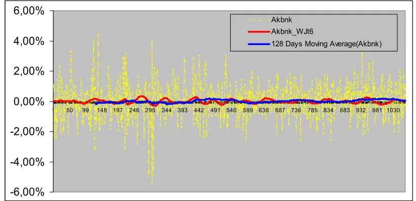
Figure nr (2) shows the comparison of 128-day daily wavelet analysis and 128-day moving average for AKBNK stock. The moving average can not get the average shock period where as wavelet analysis can do it.
-6,00% -4,00% -2,00% 0,00% 2,00% 4,00% 6,00%
1 50 99 148 197 246 295 344 393 442 491 540 589 638 687 736 785 834 883 932 981 1030
Akbnk Akbnk_WJt6
128 Days Moving Average(Akbnk)
Figure 2. 128 days time-scale(light line) and 128 days moving average(dark line) of AKBNK stock
Fourier series regulated by Sinus and Cosine functions is expressed by equation nr (5) mathematically (Tkacz, 2001:22).
∑
∞=
+
+
=
1
0
(
cos
2
sin
2
)
)
(
k
k
k
kx
a
kx
b
b
x
f
π
π
(5)b0=
∫
( )
π
π
2
0 1
dx x f 2
, bk =
∫
( )
( )
π
π
2
0 1
dx kx Cos x
f ,
ak =
∫
( ) ( )
π
π
2
0
1
dx kx Sin x f
[image:7.595.91.502.302.501.2]a0, ak and bkparameters can be solved by using the smallest squares methods.
)
2
(
)
(
1 2 0 00
c
k
c
x
f
j k jk j j−
+
=
∑
∑
− = ∞ =χ
ψ
(6)) (x
ψ is called as the base wavelet and it is the foundation of all of ψ ’s, from equation nr 7, expansion and transform (Tkacz, 2001:22).
( )
⎪ ⎪ ⎪ ⎩ ⎪ ⎪ ⎪ ⎨ ⎧ < ≤ − < ≤ = Ψ others : 0 1 2 1 : 1 2 1 0 : 1 x xx (7)
Maximal overlap discrete wavelet transform-MODWT is used in the high frequency financial time series. MODWT can be applied to any of N data set, however, wavelet variance carry asymptotic feature. This feature of MODWT allows it to be used in any given N-data set. MODWT is expressed by the matrixes (Gençay et al., 2002 and Percival and Walden, 2000). MODWT is expressed as scaled wavelet and scaling filter coefficient according to (8) and (9) equations. ) 1 ( ~ , ,
~
=∑
− = t f w N L t X t j t j jW
(8)) 1 ( ~ , ,
~
=∑
− = t f v N L t Y t j t j jV
(9)Wavelet variance of λj measurement determined by MODWT is expressed in (10) and (11) nr equations (In and Kim, 2006).
[ ]
∑
==
N L t X t j j X jW
N
v
(
)
1
~
~
, 2~
λ
(10)[ ]
∑
==
N L t Y t j Y j jV
N
v
(
)
1
~
~
, 2~
λ
(11)
4 Data and Empirical Findings
Data
Study data consist of 10 stocks from ISE 30 namely AKBNK, AEFES, AKGRT, ARCLK, EREGL, KCHOL, KRDMD, TCELL, TUPRS and YKBNK. 10 stocks are selected randomly with their data set starting from 2002 and the sample rate is 33% (10/30). The volatility changed to the scale, systematic risk and long term memory parameter were determined by
8
[image:9.595.78.519.146.355.2]wavelet theory. Data sets are obtained from the web site, www.analiz.com. The statistical characteristic of the level data of the chosen stocks can be seen in Table 1. The flatness and distortion features of all stock returns are different from each other; and it can be considered that stocks are in normal distribution according to the normality test - Jarque-Bera Test.
Table 1: Main statistical features (level series) Stock
exchange Min. Max
Std.
Deviation Skewness Kurtosis Jarque-Bera
AKBNK 14786 135103 29218.5 1.08972 3.49509 221.864 AEFES 93607 497321 97053.8 0.975298 2.94809 169.117 AKGRT 14680 145396 26896.7 1.64071 5.84979 838.987 ARCLK 21185 130137 23953.9 0.371356 2.7581 27.1002 EREGL 12199 97200 24496.7 0.708779 2.30727 110.568 KCHOL 25991 82246 13387.7 0.307466 2.16677 47.6328 KRDMD 0.0299 0.7452 0.225812 0.352008 1.44914 128.845 TCELL 16126 102214 23572.3 0.534852 1.84816 109.754 TUPRS 44665 303477 66169 1.05593 2.81388 199.636 YKBNK 10195 79864 17992.2 0.394087 2.1502 59.6686 ISE100 8627.42 47728.5 10039.8 1.01437 3.1919 184.445 ISE30 10880.5 60772.1 12882.6 0.978913 3.11851 170.877
In determination of both volatility and long term memory effect parameter, the first degree logarithmic differences of the series are taken. It is a common application in literature that 1st degree logarithmic differences are used. In the study 1st degree logarithmic differences of all series are taken.
In Table 2, there are stability values of stock returns at the level (I(0)) according to KPSS test (Kwiatkowski et al, 1992), Phillips-Peron test (Phillips and Peron, 1988) and Augmented Dickey Fuller test (Dickey and Fuller, 1981). Series are not stable at I(0) and they are stabilized when the logarithmic differences are taken according to the unit-root tests (Table 3).
Table 2. Unit Root Test (level series) Stock
exchange KPSS test I(0)
Phillips- Peron test I(1)
Augmented D-F test I(1)
AKBNK 20.0126 0.638136 0.504895
AEFES 20.456 0.389534 0.563084
AKGRT 17.512 -1.44333 -1.46362
ARCLK 20.4979 -0.218052 -0.393636
EREGL 21.6616 -0.000165 -0.0483108
KCHOL 18.6793 -0.686503 -0.838449
KRDMD 20.7315 0.047202 0.0981312
TCELL 21.8022 -0.096907 -0.0878089
TUPRS 19.7428 1.52696 1.60709
YKBNK 16.8746 0.231628 0.0857086
ISE100 20.2774 1.57173 1.63275
[image:9.595.72.518.528.721.2]9
Table 2. Unit Root Test (log differenced series) Stock
exchange KPSS test I(0)
Phillips- Peron test I(1)
Augmented D-F test I(1)
AKBNK 0.0653892* -26.694* -26.8563*
AEFES 0.2068* -27.7824* -27.9301* AKGRT 0.0795931* -30.0199* -30.011*
ARCLK 0.0331696* -25.5729* -25.7272*
EREGL 0.0941811* -25.8769* -25.9482*
KCHOL 0.0866762* -25.528* -25.6102*
KRDMD 0.123164* -26.8404* -23.9578*
TCELL 0.144187* -26.0658* -22.2537*
TUPRS 0.333554* -28.6147* -28.6611*
YKBNK 0.37495* -24.2236* -21.792*
ISE100 0.330153* -32.9528* -32.9307*
ISE30 0.309776* -33.038* -33.0119* * represents %1 C.I. statistically significance
Empirical Findings
CAPM and multiscale CAPM have been tested for 10 stocks from ISE 30. In the study, firstly, multiscale variance difference was determined.
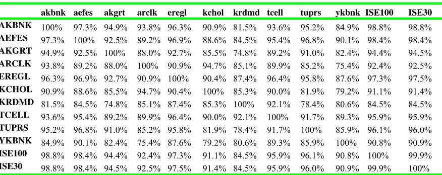
In table 4, you can see linear correlation of 10 stocks covered in the study from ISE 30. The correlation between the stocks and ISE 30 and ISE 100 is in the range of 91.4% 98.8%
Tablo 4: Linear Correlation
akbnk aefes akgrt arclk eregl kchol krdmd tcell tuprs ykbnk ISE100 ISE30 AKBNK 100% 97.3% 94.9% 93.8% 96.3% 90.9% 81.5% 93.6% 95.2% 84.9% 98.8% 98.8% AEFES 97.3% 100% 92.5% 89.2% 96.9% 88.6% 84.5% 95.4% 96.8% 90.1% 98.4% 98.4% AKGRT 94.9% 92.5% 100% 88.0% 92.7% 85.5% 74.8% 89.2% 91.0% 82.4% 94.4% 94.5% ARCLK 93.8% 89.2% 88.0% 100% 90.9% 94.7% 85.1% 89.9% 85.2% 75.4% 92.4% 92.5% EREGL 96.3% 96.9% 92.7% 90.9% 100% 90.4% 87.4% 96.4% 95.8% 87.6% 97.3% 97.5% KCHOL 90.9% 88.6% 85.5% 94.7% 90.4% 100% 85.3% 90.0% 81.9% 79.2% 91.1% 91.4%
KRDMD 81.5% 84.5% 74.8% 85.1% 87.4% 85.3% 100% 92.1% 78.4% 80.6% 84.5% 84.5% TCELL 93.6% 95.4% 89.2% 89.9% 96.4% 90.0% 92.1% 100% 91.7% 89.3% 95.9% 95.9% TUPRS 95.2% 96.8% 91.0% 85.2% 95.8% 81.9% 78.4% 91.7% 100% 85.9% 96.1% 96.0% YKBNK 84.9% 90.1% 82.4% 75.4% 87.6% 79.2% 80.6% 89.3% 85.9% 100% 90.8% 90.9% ISE100 98.8% 98.4% 94.4% 92.4% 97.3% 91.1% 84.5% 95.9% 96.1% 90.8% 100% 99.9% ISE30 98.8% 98.4% 94.5% 92.5% 97.5% 91.4% 84.5% 95.9% 96.0% 90.9% 99.9% 100%
In table 5, there are multiscale variance data for 10 stocks and ISE indices. Average multiscale variance shows the risk situation at short, mid and long term.
10
Table 5. Variance analysis with wavelets
Lower
Border(L) Variance (wavelet) Upper Border(U)
AKBNK 0.115 0.1047 0.1252
AEFES 0.0972 0.0888 0.1057
AKGRT 0.1115 0.1016 0.1214
ARCLK 0.1084 0.0987 0.1182
EREGL 0.0968 0.0881 0.1055 KCHOL 0.0932 0.0849 0.1016
KRDMD 0.2955 0.2696 0.3214
TCELL 0.1228 0.1121 0.1336
TUPRS 0.1039 0.0948 0.1131
YKBNK 0.2105 0.1918 0.2291
ISE100 0.916 0.8383 0.9936
ISE30 0.101 0.0924 0.1095
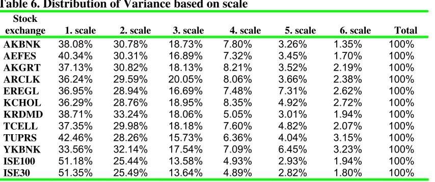
In Table 6 and Figure 3, multiscale variance distribution is available instead of average scale of variance. According to test results which are parallel to expectation, variance is increasing for all stocks as the scale increased. However it is seen that multiscale variance of YKBNK has higher multiscale variance at all scales. YKBNK has the smallest multiscale variance whereas TUPRS has the highest one at the 1st (1-4 days) scale. In the 6th scale (128 days), as the highest scale chosen, AKBNK has the smallest variance and YKBNK has the highest one. These results show that YKBNK stock has the lowest level of risk at holding periods of 1 to 4 days, while for 128 days of holding period AKBNK has the smallest risk level.
It is determined that, for the stocks chosen from ISE 30, risk levels are changing according to the multiscale variance analysis (according to stock holding periods). This finding supports the argument of “variance should be calculated multiscale (according to the stock holding period) systematic risk coefficient instead of fixed interval systematic risk coefficient (beta or value subject to variance-risk etc).”
Table 6. Distribution of Variance based on scale
Stock
exchange 1. scale 2. scale 3. scale 4. scale 5. scale 6. scale Total AKBNK 38.08% 30.78% 18.73% 7.80% 3.26% 1.35% 100%
AEFES 40.34% 30.31% 16.89% 7.32% 3.45% 1.70% 100%
AKGRT 37.13% 30.82% 18.13% 8.21% 3.52% 2.19% 100%
ARCLK 36.24% 29.59% 20.05% 8.06% 3.66% 2.38% 100%
EREGL 36.95% 28.94% 16.69% 7.48% 7.31% 2.62% 100%
KCHOL 36.29% 28.76% 18.95% 8.35% 4.92% 2.72% 100%
KRDMD 38.71% 33.24% 18.06% 5.05% 3.01% 1.94% 100%
TCELL 37.35% 29.98% 18.18% 7.60% 4.82% 2.07% 100%
TUPRS 42.46% 28.26% 15.73% 6.36% 4.04% 3.15% 100%
YKBNK 33.56% 32.14% 17.54% 7.09% 6.45% 3.23% 100%
ISE100 51.18% 25.44% 13.58% 4.93% 2.93% 1.94% 100%
[image:11.595.73.500.492.671.2]0 0,1 0,2 0,3 0,4 0,5 0,6 0,7 0,8
1 2 3 4 5 6
Time-Scale
M
u
lti-s
ca
le
V
ar
ia
n
ce
Akbnk Aefes Akgrt Arclk Eregl Kchol Krdmd Tcell Tuprs Ykbnk
İMKB100
[image:12.595.100.497.72.275.2]İMKB30
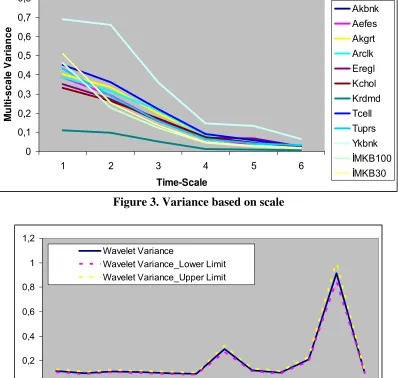
Figure 3. Variance based on scale
0 0,2 0,4 0,6 0,8 1 1,2
Akbn k
Aef es
Akgr t
Arc lk
Eregl Kcho l
Krdm d
Tcel l
Tupr s
Ykbn k
İmk b10
0
İmk b30 Wavelet Variance
[image:12.595.99.497.84.462.2]Wavelet Variance_Lower Limit Wavelet Variance_Upper Limit
Figure 4. Variance anlysis with wavelets
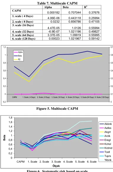
In Table 7, multiscale CAPM test results are available on average values for the 10 stocks. Systematic risk (beta) changes according to the scale. Beta averages of stocks: 0.44 in the 1st scale, 0.85 in the 2nd scale, 1.01 in the 3rd scale, 1.02 in the 4th scale, 1.09 in the 5th scale and 1.02 in the 6th scale. YKBNK and KRDM differentiate from other stocks due to their higher beta values in higher scales*. As seen in Figure 6, beta values of all stock are closing each other at the 1st scale. This situation indicates that multiscale analysis for 1 to 4 days may not be adequate. The approaching to “1” of systematic risk after the 3rd scale (8 to 16 days) supports the argument “CAPM should be tested at the scales later than 8 to 16 days.”
Table 7. Multiscale CAPM
Alpha Beta R2
CAPM
0.000182 0.707044 0.37676
1. scale ( 4 Days)
4.06E-06 0.443118 0.25994
2. scale ( 8 Days) 0.0232 0.856786 0.47105
3. scale (16 Days)
4.47E-05 1.0126 0.55994
4. scale (32 Days) -6.9E-07 1.021196 0.49827
5. scale (64 Days) 3.37E-05 1.09919 0.55995
6. scale (128 Days) 0.00023 1.021967 0.59142
-0,2 0 0,2 0,4 0,6 0,8 1 1,2
CAPM 1. Scale ( 4 Days) 2. Scale ( 8 Days) 3. Scale (16 Days) 4. Scale (32 Days) 5. Scale (64 Days) 6. Scale (128 Days) 0 0,1 0,2 0,3 0,4 0,5 0,6 0,7 Alpha
Beta R2
Figure 5. Multiscale CAPM
0 0,2 0,4 0,6 0,8 1 1,2 1,4 1,6 1,8
CAPM 1. Scale 2. Scale 3. Scale 4. Scale 5. Scale 6. Scale
Ölçek
Be
ta
Akbnk Aefes Akgrt Arclk Eregl Kchol Krdmd Tcell Tuprs Ykbnk
Figure 6. Systematic risk based on scale
12
In Figure 7, there is a relationship between multiscale return and systematic risk coefficients (beta). The finding related to beta and return to be in better form determined by Gencay et
al(2005) in a study conducted in International indices are not applicable for ISE 30. Risk and
-0,070% -0,060% -0,050% -0,040% -0,030% -0,020% -0,010% 0,000% 0,010% 0,020%
0 0,1 0,2 0,3 0,4 0,5 0,6 0,7 0,8 0,9
Beta A ver ag e R et u rn 0,000% 0,000% 0,000% 0,000% 0,000% 0,000%
0 0,2 0,4 0,6 0,8 1 1,2
Beta A ver ag e R et u rn
D0 D1
-0,001% -0,001% -0,001% -0,001% 0,000% 0,000% 0,000% 0,000% 0,000% 0,000% 0,000%
0 0,2 0,4 0,6 0,8 1 1,2
Beta A ve rag e R et u rn -0,002% -0,002% -0,001% -0,001% -0,001% -0,001% -0,001% 0,000% 0,000% 0,000%
0 0,2 0,4 0,6 0,8 1 1,2 1,4
Beta A ve rage R et u rn
D2 D3
-0,002% -0,001% -0,001% 0,000% 0,001% 0,001% 0,002% 0,002%
0 0,2 0,4 0,6 0,8 1 1,2 1,4
Beta A ve rage R et u rn -0,002% -0,002% -0,001% -0,001% 0,000% 0,001% 0,001% 0,002% 0,002%
0 0,2 0,4 0,6 0,8 1 1,2 1,4 1,6 1,8
Beta A ve rage R et u rn
D4 D5
-0,001% -0,001% 0,000% 0,001% 0,001% 0,002% 0,002% 0,003% 0,003% 0,004% 0,004%
0 0,2 0,4 0,6 0,8 1 1,2 1,4 1,6 1,8
Beta A ver ag e R et u rn D6
* D1: 1.scale(1-4 days), D2: 2.scale(5-8 days), D3: 3.scale(9-16 days), D4: 4.scale(17-32 days), D5: 5.scale(33-64 days), D6: 6.scale(65-128 days)
14
Figure 7. Average return and beta based on scale 5 Conclusion and Recommendations
In this study, Wavelets method, as a new analysis method in finance and economics, and multiscale variance and multiscale Capital Asset Pricing Model (CAPM) were tested. Multiscale variance as a general risk indicator and multiscale CAPM as a systematic risk indicator brought a new approach to portfolio theory. In this study, variance and systematic risk change according to the scale have been determined for 10 stocks from ISE 30. The ability of the investors to conduct risk based analysis up to 128 days allows them to determine the risk level to the scale (stock holding period).
According to the study results; it is determined that the variances of 10 stocks from ISE 30 change according to the scale and variance differentiation as an expression of general risk level increase starting from the 1st scale (1 to 4 days).
In multi-scale CAPM, it is determined that systematic risk of all stocks is changed to frequency (scale) and increased at higher scales. The finding as to beta and return at the high levels to be in stronger form evidenced by Gencay et al (2005) is determined as not applicable to ISE 30. The risk and return for ISE 30 are close to the positive in the 3rd scale (32 days), but they are in the same direction for the other scales. This finding shows that the risk-return maximization of a portfolio of 10 stocks from ISE may be achieved at a level of 32 days and the risk will be higher than the return in the portfolios established at those levels different than 32 days.
References
Albora, A.M., Ucan, O.N., Hisarlı, Z.M., Stümpel, H., “Sivas-Kuşaklı Uygarlığının Dalgacık Yöntemi Kullanılarak Arkeo-Jeofizik Araştırılması”, Uygulamalı Yerbilimleri Dergisi, Cilt 2,
Sayı 1, 2002, ss.59-69
Almasri, A. and Shukur, G., “An Illustration of the Causality Relationship Between Government Spending and Revenue Using Wavelets Analysis on Finnish Data”, Journal of Applied Statistics, 30(5), 2003, ss.571-584
Ang, A., and J.Chen, “Asymmetric Correlations of Equity Portfolios”, Journal of Financial Economics, 63, 2002, ss. 443-494.
Aytaç, U., Dalgacıklar Teorisi, Bitirme Projesi, ITU Mühendislik Fakültesi, Matematik Bölümü, 2004.
Brailsford T.J. and Faff, R.W., Testing the conditional CAPM and the effect of intervaling: a note, Pacific-Basin Finance J. 5, 1997, ss.527–37,
Brailsford, T.J. and Josev, T, The impact of return interval on the estimation of systematic risk Pacific-Basin Finance J. 5, 1997, ss.353–72
15
Çetin,U., Kucur,O.; "Dalgacık Dönüşümü Metodu İle Deprem İşaretlerinde Faz Geliş Zamanlarının Tesbiti," 11. Sinyal İşleme Ve İletişim Uygulamaları (SİU) Kurultayı, İstanbul, 18-20 Haziran, 2003a.
Çetin,U., Kucur,O.; "Dalgacık Dönüşümü Metodu İle Faz Geliş Zamanlarının Tesbiti," 5. Ulusal Deprem Mühendisliği Konferansı, İstanbul Teknik Üniversitesi, 26-30 Mayıs, 2003b
Dalkir, M., “A new approach to causality in the frequency domain, Economics Bulletin”, Economics Bulletin, 3(44), 2004, ss. 1-14
Daubechies, I., “Ortonormal bases of compactly supported wavelets”, Communications on Pure and Applied Mathematics, 41, 1988, ss.909-996
Dickey, D.A. and Fuller, W.A., “Likelihood ratio statistics for an autoregressivetime series with a unit root”, Econometrica, 55, 1981, ss.251-276
Dirgenali F, and Kara S, “Yapay Sinir Ağları Ve Dalgacık Dönüşümü Kullanılarak Damar Sertliği Hastalığının Teşhisi”, Biyomedikal Mühendisliği Ulusal Toplantısı (BİYOMUT’05), 25-27 Mayıs, 2005.
Fernandez, V.P., “The international CAPM and a wavelet-based decomposition of value at risk”, Studies in Nonlinear Dynamics and Econometrics, 9(4), 2005, ss. 83-119
Fernandez, V., “The CAPM and value at risk at different time-scales”, International Review of Financial Analysis, 15(3), 2006, ss.203-219
Frankfurter G., Leung, W. and Brockman, W., “Compounding period length and the market model”, J. Economics Business, 46, 1994, ss.179–93
Gallegati, M., "A Wavelet Analysis of MENA Stock Markets," Finance 0512027, Econwpa,2005a,Http://İdeas.Repec.Org/P/Wpa/Wuwpfi/0512027.Html,[Erişim:27.03.2006 ]
Gallegati, M., “Stock Market Returns and Economic Activity: Evidence from Wavelet Analysis”, Mimeo, DEA and SIEC, Universit Politecnica dele Marche, 2005b
Gallegati, M. and Gallegati, M., “Wavelet Variance and Correlation Analyses of Output in G7 Countries”, Mimeo, DEA, Universit Politecnica dele Marche, 2005
Gençay, R., Selcuk, F., Whitcher, B., An Introduction to Wavelets and Other Filtering Methods in Finance and Economics(Academic Pres), 2002
Gençay, R., Selcuk, F., Whitcher, B., “Systematic risk and timescales”, Quantitative Finance, 3 (2), 2003, ss.108-116
Gençay, R., Selcuk, F., Whitcher, B., “Multiscale systematic risk”, Journal of International Money and Finance, 24 (1), 2005, ss. 55-70
16
Handa, P., Kothari, S.P. and Wasley, C., “The relation between the return interval and betas: implications for the size effect”, J. Financial Economics, 23, 1989, ss.79–100
Handa, P., Kothari, S.P. and Wasley, C., “Sensitivity of multivariate tests of the capital asset pricing to the return interval measurement”, J. Finance, 48, 1993, ss.15–43
In, F. and Kim, S. “The Hedge Ratio and the Empirical Relationship Between the Stock and Futures Markets: A New Approach Using Wavelets”, The Journal of Business, 79, 2006, ss.799-820
Kara, S., Dirgenali, F., and Okkesim, Ş., “Diyabetli Hastalarda Düzensiz Mide Ritimlerinin Dalgacık Dönüşümü Kullanılarak Teşhisi”, Biyomedikal Mühendisliği Ulusal Toplantısı (BİYOMUT’05), 25-27 Mayıs, 2005
Kim, S., and In, H.F., “The Relationship Between Financial Variables and Real Economic Activity: Evidence from Spectral and Wavelet Analyses”, Studies in Nonlinear Dynamic&Econometrics, 7( 4), 2003
Kim, S. and In, F., “The relationship between stock returns and inflation: new evidence from wavelet analysis”, Journal of Empirical Finance, 12(3), 2005a, ss.435-444
Kim, S., and In, F., “Multihorizon Sharpe ratio.” Journal of Portfolio Management 31, 2005b, ss.105-101
Kim, S. and In, F., “On the relationship between changes in stock prices and bond yields in the G7 countries: Wavelet analysis”, Journal of International Financial Markets, Institutions and Money, 17(2), 2007, ss.67-179
Kwiatkowski, D., Phillips, P. C. B. , Schmidt, P. and Shin, Y. “Testing the null hypothesis of stationarity against the alternative of a unit root”, Journal of Econometrics, 54, 1992, ss.159-178.
Lee, H.S., “International transmission of stock market movements: a wavelet analysis”, Applied Economics Letters, 11(3/20), 2004, ss.197-201
Lin, S. and Stevenson, M., “Wavelet analysis of the cost-carry model”, Studies in Nonlinear Dynamic&Econometrics, 5( 1), 2003, ss.87-102
Lintner, J., “The valuation of risk assets and the selection of risky investments in stock portfolios and capital budgets”, Review of Economics and Statistics, 47, 1965, ss.13-37.
Mallat, S., “A theory for multiresolution signal decomposition: The wavelet representation”, IEEE Transactions on Pattern Analysis and Machine Intelligence, 11, 1989, ss.674-693
Mossin, J., Equilibrium in a Equilibrium in a Capital Asset Market, Econometrica, 34, ss.68-83.
17
Percival, D.B. and Walden, A.T., Wavelet Methods for Time Series Analysis(Cambridge University Pres), 2000
Phillips, P.C.B. and Peron, P. “Testing for a Unit Root in Time Series Regression,” Biometrika, 75, 1988, ss.335–346.
Ramsey, J.B. and Lampart, C., “Decomposition of Economic Relationships by Timescale Using Wavelets”, Macroeconomic Dynamics, 2(1), 1998, ss.49–71
Robinson, P. M., “Log-periodogram regression of time series with long-range dependence”, Annals of Statistics 23, 1995, ss.1048–1072.
Roll, R., “A Critique of the Asset Pricing Theory’s Tests; Part I: On Past and Potential Testability of the Theory”, Journal of Financial Economics, 4, 1977, ss. 129-176.
Sharpe, William F., “Capital asset prices: A theory of market equilibrium under conditions of risk”, Journal of Finance, 19 (3), 1964, ss.425-442.
Selçuk, F., Dalgacıklar: Yeni Bir Analiz Yöntemi, Bilkent Dergisi, Mart, 2005
Okkesim, Ş., Kara, S., Uysal, T., and Yağcı,, A., “Pre-Ortodontik Trainer Aparesi Kullanılan Hastalarda Çene Kaslarının Elektromyogram ve Ayrık Dalgacık Dönüşümü İle Analizi”, Biyomedikal Mühendisliği Ulusal Toplantısı (BİYOMUT’06), İstanbul, 25-28,Mayıs, 2006
Ulusoy, I., Halıcı, U., Karakaş, S., Leblebicioğlu, K., and Atalay, V., İşitsel Uyarılar Sonucu Oluşan EEG Sinyallerinin Dalgacık Dönüşümü Kullanılarak Yapay Sinir Ağları İle Sınıflandırılması, 7.Sinyal İşleme Ve Uygulamaları Kurultayı (SİU'99), 1999, s.386-390.
Özün, A. and Çifter, “Bankaların Hisse Senedi Getirilerinde Faiz Oranı Riski: Dalgacıklar Analizi ile Türk Bankacılık Sektörü Üzerine Bir Uygulama”, Bankacılar Dergisi, Sayı 59,
2006, ss.1-15
Treynor, Jack, “Towards a theory of market value of risky assets”, unpub. manuscript, 1961