Munich Personal RePEc Archive
An Inflated Ordered Probit Model of
Monetary Policy: Evidence from MPC
Voting Data
Brooks, Robert and Harris, Mark and Spencer, Christopher
August 2007
An In
fl
ated Ordered Probit Model of Monetary
Policy: Evidence from MPC Voting Data
∗
Robert Brooks
†Mark N. Harris
‡Christopher Spencer
§August 2007
Abstract
Even in the face of a continuously changing economic environment, interest rates often remain unadjusted for long periods. When rates are moved, the norm is for a series of small unidirectional discrete basis-point changes. To explain these phenomena we suggest a two-equation system combining a “long-run” equation explaining a binary decision to change or not change the interest-rate, and a “short-run” one based on a simple monetary policy rule. We account for unobserved heterogeneity in both equations, applying the model to unique unit-record level data on the voting preferences of Bank of England Monetary Policy Committee (MPC) members.
JEL Classification: C3, E50.
Keywords: Interest rates, voting, discrete data, ordered models, inflated outcomes.
∗We wish to thank Max Gillman, Paul Levine, and seminar participants at the Banque de France, the
University of Queensland, Melbourne University and the University of Surrey. The usual caveats apply. †Professor of Econometrics, Department of Econometrics and Business Statistics, Monash University, Australia. e-mail: [email protected]
‡Associate Professor, Department of Econometrics and Business Statistics, Monash University, Aus-tralia. e-mail: [email protected]
§Research Fellow, Department of Economics, University of Surrey, UK. e-mail:
1
Introduction
Inflation rate targeting by autonomous central banks via manipulations of short-term
in-terest rates is a defining characteristic of monetary policy in many industrialized countries,
as is the observation that for many countries - consider the Bank of England in the UK
- decisions on interest rate policy are undertaken by committees (Fry, Julius, Mahadeva,
Roger, and Sterne 2000)
Yet just as the institutional frameworks for monetary policy in industrialized countries
have broadly defined characteristics, so too does the behaviour of short-term interest rates.
Much modern monetary policy is characterized by three highly related stylized empirical
regularities: interest rate inertia, stepping, and gradualism. Inertia relates to the fact
that even with the arrival of new economic information, interest rates are infrequently
adjusted. For example, Riboni and Ruge-Murcia (2006) consider recent interest rate
decisions by the U.S. Federal Reserve, the European Central Bank, the Bank of England
and the Bank of Canada, respectivelyfinding that approximately55,90,70and40percent
of observations correspond to no-change in short-term rates. A related phenomenon,
interest rate stepping, is that when ratesaremoved, they are done so in a series of discrete
intervals, typically 25basis point multiples ranging from −75to75 basis points. Finally,
gradualism refers to the fact that when rates are changed, they are moved in a series of
small steps rather than fewer relatively larger ones. Accordingly, although it is possible
to observe one-off changes in the order of 50 basis points or more, the overwhelming
majority of changes follow a series of unidirectional discrete 25 basis-point adjustments.
Such a phenomenon is also often referred to as smoothing (Verhagen 2002). Due to their
complementarity, some authors definestepping as the combination ofinertia andstepping
as defined above (Clerc and Yates 1999). To summarize, rates are often not moved in the
face of a changing economic environment, and if they are so, they are typically moved in
a series of small discrete steps.
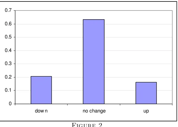
To illustrate these points,Figure 1plots the data on which the empirical estimations
are subsequently based: the short term interest rate (rate on repurchase agreements,
known as the repo-rate) decided on at each of the Bank of England’s Monetary Policy
Committee (MPC) monthly meetings since June 1997. Clearly, this series is dominated
0 1 2 3 4 5 6 7 8 Jun-9 7 Dec-97 Jun-9 8 Dec-98 Jun-9 9 Dec-99 Jun-0 0 Dec-00 Jun-01 Dec-01 Jun-0 2 Dec -02 Jun-0 3 Dec-03 Jun-0 4 Dec-04 Jun-0 5 Dec-05
Interest Rate / Inflation / Target Inflation (%)
Interest Rate RPIX Target CPI Target CPI Inflation RPIX Inflation
June 1997 - Dec 2003: MPC given responsibility for setting interest rates and hitting inflation target of RPIX 2.5%
[image:4.595.106.526.101.368.2]Jan 2004 - : Target changed to 2% CPI inflation
Figure 1.
MPC Interest Rate Decisions, RPIX and CPI Inflation Targets and corresponding Inflation levels, June 1997-May 2006
are characterized by small, discrete, amounts. Indeed, in this period, there were only two
(absolute) observed interest rate movements, of respectively, 0.25and 0.5 basis points.
In this paper, we utilize an infrequently used data set relating to the voting decisions of individual committee members of the MPC of the Bank of England. The repeated
ob-servations for each member allow us to condition on the likely presence of any unobserved
heterogeneity of the individual members. However, the major contribution of the current
paper lies in the empirical estimation of members’ interest rate preferences which
simul-taneously allows for a “long-run” (or inertia) equation with a “short-run” (or adjustment)
one. This system of equations allows one to “inflate” the probability of a “no-change”
decision on interest rate levels; and moreover, to allow such observations to arise from two
distinctly different siutations. This is based both on recent theoretical literature which
attempts to explain the empirical bias towards such inertia, and also on this empirical phenomenon directly. The estimation strategy also allows for the remaining two stylized
facts of stepping andgradualism. In so doing, we develop a new econometric model that
2
Literature
Dating back to Taylor (1993), a great deal of recent literature characterizes monetary
policy as being based on a set of simple “rules”. The so-calledTaylor rule postulates that
policy makers condition short term interest rates positively on the gap between target and
actual inflation, and similarly to the output gap; and, although anecdotally many central
bankers deny use of such policy rules, estimated equations based on such appear to provide a very good description of the data: see, for example, Clarida, Gali, and Gertler (2000).
Yet as noted by Carare and Tchaidze (2005) much of the empirical methodology employed
in the estimation of such rules is characterized by a times series approach: specifically,
the application of OLS to backward looking rules (Orphanides 2001) or of GMM and IV
techniques to forward looking ones, such as Clarida, Gali, and Gertler (2000) and more
recently Jondeau, Le Bihan, and Galles (2004). There has also been a significant amount
of theoretical literature attempting to provide an economic framework for monetary policy
inertia. However, as the current paper is primarily an empirical piece, wefirst concentrate
on the empirical literature before turning to recent theoretical contributions.
A number of empirical studies have applied limited dependent variable techniques
to modelling official interest rate setting. Eichengreen, Watson, and Grossman (1985)
model the setting of the bank rate by the Bank of England in the interwar gold standard
period using a dynamic probit model. Davutyan and Parke (1995) extend this approach
by applying a dynamic probit model to the setting of the bank rate in the period prior
to World War I. Hamilton and Jorda (2002) propose a different approach to modelling
the US federal funds target rate over the period from 1984 to 2001. Specifically, they
extend the autoregressive conditional duration model (Engle and Russell 1997, Engle and
Russell 1998) to model the likelihood that the target rate will change tomorrow, given the available information set today (the Hamilton and Jorda (2002) model also includes
an ordered probit component). Dolado and Maria-Dolores (2002) provide an alternative
in the framework of a marked-point-process approach by applying a sequential probit
model to understand the interest rate policy of the Bank of Spain for the period 1984 to
1998. Dolado and Maria-Dolores (2005) also employ an ordered probit approach to study
the interest rate setting behaviour of four European central banks and the US Federal
As in this paper, other studies have utilized information contained in the MPC’s voting
record. Spencer (2006) adopts a related approach to the current paper, using a similar
dataset and discrete choice methods. Simple ordered probability models are estimated
although the focus is mainly on the inherent differences between the voting behaviour of
“internal” and “external” MPC members. Similarly, Bhattacharjee and Holly (2005) also
use the same data on Bank of England MPC member voting intentions, exploiting the
heterogeneity in members’ votes to shed light on the main determinants of MPC decisions.
Bhattacharjee and Holly (2005) also allow for a distinction between internal and external MPC members in their estimation approach.
The internal/external distinction is also followed in Gerlach-Kristen (2003) who shows
that disagreements between members of the Bank’s MPC typically constitute the rule,
and not the exception. In a further paper (Gerlach-Kristen 2004), it is shown that future
changes in the short term rate can be predicted utilizing voting record information. This
is achieved through using a measure called skew, which proxies for the extent to which
MPC members disagree with each other at a given meeting. Financial market participants
are shown to respond to the release of the voting record, suggesting the transparency of
UK monetary policy is enhanced by its publication.
Given that we are utilizing voting data, this paper is also related to a literature which
is geared towards explaining the voting behaviour of members of the United States FOMC.
As we generally model MPC members’ votes as a function of theeconomic environment, it
falls into what Meade and Sheets (2005) label the “reaction function” camp (Tootell 1991b,
Tootell 1991a), and not the “partisan theory of politics” genus of studies (see, for example,
Belden 1989, Havrilesky and Schweitzer 1990, Havrilesky and Gildea 1991).1 In much
the same way as we distinguish between internal and external members, FOMC studies
distinguish Federal Reserve Board Members from Reserve Bank Presidents, with a view
to identifying differences in the voting behaviour of members belonging to both groups.
Tootell (1991b) tests the hypothesis that District Bank Presidents set policy according to
regional, as opposed tonational economic conditions. No evidence to support this claim is found, although evidence to the contrary is found by Meade and Sheets (2005). As
MPC members should not be seen as providing regional representation this hypothesis is
not pursued here. In a further paper, Tootell (1991a) tests, but fails to find evidence, to support the hypothesis that Federal Reserve Bank Presidents vote more “conservatively”
than Board Governors. Specifically, the voting behaviour of Reserve Bank Presidents is
found to be no different to Board members. In both contributions, Tootell (1991b) and
Tootell (1991a) use forward looking variables in the form of Greenbook estimates of GDP
growth and inflation as covariates. Given that the economy is influenced with lags by
monetary policy, it follows that FOMC members’ votes are most likely determined by
their expectations of inflation and GDP growth. In all cases, estimations are performed
using standard econometric techniques such as multinomial logits and probits.
In terms of theoretical contributions, a useful starting point is Verhagen (2002) who
discusses empirical shortcomings of dynamic models of monetary policy: in studies such
as Svensson (1997), while some inertia can be instigated into the system through allowing
the central bank to care about the output gap, the central bank’s instrument typically
reacts immediately to any change in the determinants of future inflation. Policy does not
thus remain unchanged in a changing economic environment, and the policy instrument
does not move in fixed-sized increments. The model of Svensson (1997) thus typifies
models of interest rate determination which cannot explain the stylized empirical facts of interest rate setting such as inertia and stepping.
Institutionally, rates are typically only changed at the regular (often monthly)
deci-sion meetings of the central bank. Effectively this places an upper bound of the number
of possible rate changes per year (although some rate changes do occur outside of these
regular meetings). However, given that the economic environment will have undoubtedly
changed since the last meeting, this begs the question of why is it likely that rates will not
be changed in light of these new developments? There a been a growing interest in the
literature concerned at trying to explain this observed empirical regularity of interest rate
inertia. Useful summaries are provided in Clerc and Yates (1999) and Verhagen (2002).
The former contribution offers explanations for stepping (where stepping refers to “the
tendency for nominal rates to stay fixed when the environment is changing; and the
ten-dency for nominal rates to move in jumps when the environment moves continuously” p.2)
under four major headings: short rate as a lever;menu costs;signalling; anduncertainty
strategic andtactical motives).
The short rate as a lever argument stems back to Goodfriend (1991) who argues that
long term rates are a more significant determinant of aggregate demand. Moreover, to
influence these, via the term structure of interest rates, one needs to affect the future
stream of expected future rates, which, in turn, is achieved by announcing fixed targets
for the short term rate over “significant” periods of time.
The menu cost argument assumes that, as with more traditional prices, there are costs
imposed on the economy in changing the cost of money. These include the costs involved in
the utilization of the central bank’s resources; incurred by agents locked intofixed interest
rate contracts; imposed by the instability in financial markets instigated by frequent
changes; and finally, frequent rate changes, especially reversals, impose costs in that they
instigate downward notions of the private sector’s competence of the central bank. Such
menu cost arguments have been formalized by Eijffinger, Schaling, and Verhagen (1999).
Charles Goodhart (a MPC member observed in the empirical example below) has stressed
the psychological motivations for such menu costs, and their importance in the decision
making process (Goodhart 1999).
The signalling approach is based on the assumption that private agents have imperfect information concerning the current monetary stance. Agents can only perceive changes
in the monetary stance in instances where changes are “large”, or at least larger than
some threshold value. A successful signal would be maximized by stepping: a jump in
rates which is then maintained for a period of time. The size of the jump required for a
successful signal might be related to the amount of recent noise in rates: a long period of
“quiet” rates, might only require a relatively small jump in rates to successfully signify a
change in monetary stance. Moreover, on the assumption that smaller, more continuous
changes are less politically costly, such stepping may increase credibility of the central
bank, by distancing itself from any potential political motives.
Afinal set of reasons for stepping relates to the assumption that central bankers incur
costs if they have to subsequently make rate reversals: the central banker waits to move
rates until the likelihood of a subsequent rate reversal is minimized. Arguments for these
reasons have been forwarded by, amongst others, Rudebusch (1995) and Goodhart (1996)
Credibility arguments have also been advanced by Rogoff (1985) and Eijffinger and
Ver-hagen (1999). More recently, Riboni and Ruge-Murcia (2006) combine a heterogeneous
committee structure with associated utility functions in a dynamic voting game to
gen-erate a bias towards inertia. As noted above, Bhattacharjee and Holly (2005) utilize a
member-specific loss-function combined with uncertainty about the economy which again
generates a bias towards no-change in policy.
3
Background: The MPC and the UK Monetary
Pol-icy Framework
The framework for UK monetary policy is embodied in the Bank of England Act 1998,
detailed accounts of which are given in Rodgers (1997), Budd (1998) and Rodgers (1998).
It is the piece of legislation accountable for (i) granting operational responsibility for
monetary policy to the Bank of England and (ii) establishing the Bank’s nine member
Monetary Policy Committee. Operational independence ensures that the Bank, and not
the Government, controls the short-term interest-rate as the key operating target of
mone-tary policy. The policy instrument used by the MPC is the rate on repurchase agreements,
more commonly known as therepo-rate. It is estimated that changes in the repo-rate take
two years to maximally impact inflation, and approximately one year for GDP.
The primary objective of monetary policy is price stability, which assumes the form of
a government inflation target. Chosen by the Chancellor of the Exchequer, this stood as
a 2.5%year on year increase in RPIX inflation for the period June 1997-December 2003,
thereafter Chancellor (Gordon Brown) announced a new target of 2% year on year CPI
inflation (seeFigure 1). The inflation target represents the “(inflation) rate at which the
MPC is required to achieve and for which it is accountable”.2 If inflation deviates by more
than 1 percentage point either side of its target, the Governor is required to write an open
letter to the Chancellor explaining “why inflation was adrift, how long the divergence was
expected to last, and the action taken to bring it back on course.” (Rodgers 1997).
Of the nine members of the MPC, five are chosen from the ranks of Bank staff
(‘in-siders’), and the remaining four are selected from external organisations (‘out(‘in-siders’),
typically from the private sector and academia. The government plays a role in the
ap-pointment of all MPC members. Decisions on the interest-rate are taken on the first
Thursday of each month and taken by simple majority rule: here, members vote on a
motion tabled by the Governor of the Bank, whose role also extends to chairing MPC
proceedings. Under the current operational monetary policy framework, the bank is
re-quired to publish a quarterly Inflation Report and the Minutes of MPC Meetings. The
Minutes, which are published two weeks after an MPC meeting, report the individual votes of MPC members.
In addition to output and inflation projections which lie at the heart of the quarterly
Inflation Report, MPC members are presented with a wide range of data upon which to
base a policy decision. This is reflected in the Minutes, which contains sections on the
“world economy”, “demand and output”, “money, credit and asset prices” and “prices
and costs”. Data on consumer confidence, changes in monetary aggregates (M0, M4),
consensus forecasts of inflation and output, industrial production and exchange rates are
invariably referred to in these sections. Of special importance is the role of the so-called
‘pre-MPC’ meeting which takes place on the Friday before a decision is taken. At such
meetings, Bank staffpresent various data and analyses which pertain to regional, national
and international economic developments. Figure 1, shows that the MPC we succcessful
in achieving its objectives in itsfirst nine years: RPIX and CPI inflation were stable and
remained close to their respective target rates of2.5%and2%, and crucially, inflation did
deviate from its target rate to trigger a open letter of explanation to the Chancellor.
4
Statistical Model
Following the much of the recent empirical literature (see, for example, Tootell 1991b,
Tootell 1991a, Spencer 2006), a discrete choice approach is adopted by re-classifying the
choice faced by members of the MPC totighten, loosen or leave interest ratesunchanged.
Such an approach, of turning a continuous variable into a discrete one, is in line with
notions of stepping: we are not concerned with the absolute value of the rate decision, just
the overall monetary stance such that we do not directly model the interest rate. Given
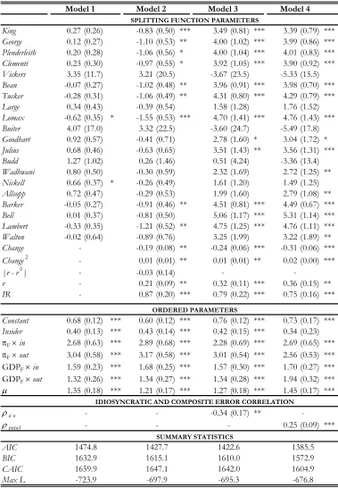
the nature of the re-classified variable, an ordered probit (OP) analysis might appear
0 0.1 0.2 0.3 0.4 0.5 0.6 0.7
[image:11.595.165.464.96.310.2]dow n no change up
Figure 2.
Empirical Distribution of Relative Voting Outcomes Frequencies
use in their rate decisions (see, for example, Spencer 2006). However, Figure 2plots the
empirical distribution of the MPC members’ stances in the sample period under study.
As noted anecdotally above, the build-up of “no-change” observations is clearly evident.
This indicates thatfirstly the standard OP is evidently not the correct statistical tool, and
secondly that the MPC possibly consider two implicit decisions revealed in their voting
intentions.
The starting point for the econometric specification employed here is an underlying
latent variable,q∗
it for each MPC memberi, at meetingt,which is a (linear in parameters)
function of a vector of observed characteristicsxit,with unknown weightsβand a random
error termuit.This latent variable represents a propensity to change equation, which can
be expressed as
qit∗ =x0
itβ+uit, (1)
where, under the assumption of normality, the probability that the MPC member sees a
justification for a change in rates is (Maddala 1983)
Pr(qit = 1|xit) = Pr(qit∗ >0|xit) =Φ(x
0
itβ), (2)
and, by symmetry, for no-change
Pr(qit= 0|xit) = Pr(qit∗ ≤0|xit) = 1−Φ(x
0
whereΦ(·)represents the standard normal cumulative distribution function. That is,this index function must be positive before a change is seen as warranted.
As documented above, this propensity for no-change is clearly evident in central bank
policy worldwide, and numerous reasons for such have been documented in previous
sec-tions. It is also possible to view this propensity to change equation as a member’s
“long-run” position, such that (potential) change is only warranted if current rates are “far
enough” from their “long-run” position and/or the current economic environment
dic-tates such.
As it stands however, equation (1) does not allow members tofine-tune this long-term
position in light of contemporaneous economic information. Moreover, even though a
member may have a long-run propensity for change, current economic conditions (the
extent of any target deviation in inflation, economic growth forecasts, and the like) may
dictate that no short-run change in current rates is, in some sense, optimal. This suggests
a two-regime scenario where the differing regimes split members into an implicit change
(qit= 1) or no-change (qit= 0) dimension - equation (1); for those in regime qit = 0, we
observe a no-change outcome; for those in the alternative regime qit= 1,we may witness
a vote for a reduction, or no-change or increase, depending on the prevailing economic
conditions. Here a no-change vote may result if forecast inflation is very close to target
levels, even though the member may have a long-run propensity for change as current
rates may be divergent from his/her notions of a preferred rate is.
The ordered probit (OP) forms the basis of the estimation strategy for regime 1
out-comes. Without loss of generality, define outcomes as yit = 0 (a rate reduction vote);
yit = 1 (no-change); and yit = 2 (increase). Conditional on being in regime 1, an
under-lying latent variable yit∗ can be specified as a linear (in parameters) function of a vector
of observed characteristics zit, with unknown weights γ and a random disturbance term
εit, thus
y∗it=z
0
itγ+εit. (4)
We therefore have that conditional on being in regime 1 (qit = 1), yit is related to this
latent variable and a boundary, or cut-off, parameter µas
yit =
⎧ ⎨ ⎩
0 if y∗
it ≤0,
1 if 0< yit∗ ≤µ, 2 if µ≤y∗
it,
where the generalizations to more outcomes are obvious. Under the unrestrictive
assump-tion of normality of εit the associated probabilities of being in each state j (j = 0,1,2)
are (Maddala 1983)
Pr(yit) =
⎧ ⎨ ⎩
Pr (yit = 0|zit, qit = 1) =Φ(−z0itγ)
Pr (yit = 1|zit, qit = 1) =Φ(µ−z0itγ)−Φ(−z
0
itγ)
Pr (yit = 2|zit, qit = 1) = 1−Φ(µ−z0itγ).
(6)
However, these probabilities are conditional on regime, qit = 1.
Under the assumption that ε and u identically and independently follow standard
Gaussian distributions, the full probabilities for y, unconditional on regime, are given by
Pr(yit) =
⎧ ⎨ ⎩
Pr (yit = 0|zit,xit) =Φ(x0itβ)Φ(−z
0
itγ)
Pr (yit = 1|zit,xit) = [1−Φ(x0itβ)] +Φ(x
0
itβ) [Φ(µ−z
0
itγ)−Φ(−z
0
itγ)]
Pr (yit =J|zit,xit) =Φ(x0itβ) [1−Φ(µ−z
0
itγ)].
(7)
In this way, along the lines of the zero-inflated Poisson (ZIP) count models (see, for
example, Mullahey 1986, Heilbron 1989, Lambert 1992, Greene 1994, Pohlmeier and Ulrich
1995, Mullahey 1997) the probability of a no-change outcome has been inflated. That is,
to observe a yit= 1 (no-change) outcome we require either that qit= 0 (the member has
a long-run no-change stance) or jointly that qit = 1 and 0< yit∗ ≤µ.
Note that this statistical model is similar in spirit to that proposed by Harris and Zhao
(2004) in the context of an OP model, except here the inflated outcome is not at one end
of the outcome spectrum. Indeed, we can further generalize this model by following Harris
and Zhao (2004) and allowing for a correlation between εanduwhich is likely ona priori
grounds as these equations relate to the same individual. Accordingly probabilities are now given by
Pr(yit) =
⎧ ⎪ ⎪ ⎨ ⎪ ⎪ ⎩
Pr (yit = 0|zit,xit) =Φ2(x0itβ,−z0itγ;−ρεu)
Pr (yit = 1|zit,xit) = [1−Φ(x0itβ)] +
½
Φ2(x 0
itβ, µ−z
0
itγ;−ρεu)
−Φ2(x 0
itβ,−z
0
itγ;−ρεu)
¾
Pr (yit = 2|zit,xit) =Φ2(x0itβ,z0itγ−µ;ρεu)
(8)
where Φ2(a, b;ρ)denotes the cumulative distribution function of the standardized
bivari-ate normal distribution with correlation coefficientρεu between the two univariate random
elements. Treating each observation as independent random draws from the population,
estimation in both instances of probabilities of the form (7) or (8), is obtained by
maxi-mizing the likelihood functionL(θ)with respect to the parameter vectorθ,θ= (β0
,γ0
andθ = (β0
,γ0
,µ, ρεu)0 respectively, where
L(θ) =
N
X
i=1
Ti
X
t=1
J−1=2
X
j=0
dijtln [Pr (yit =j|xit,zit)] (9)
where dijt is the indicator function such that
dijt =
½
1 if individual ichooses outcome j
0 otherwise. i= 1, ..., N; j = 0,1,2, t= 1..., Ti, (10)
We term these new econometric models an Inflated Ordered Probit (IOP) and
corre-lated Inflated Ordered Probit (CIOP), respectively. We also note that such models are
likely to be of use in a number of other applied situations, where there is inertia in the
observed outcomes.
Note that the system of equations (1) and (4) can be thought of as long-run and a
short-run adjustment equations, respectively, akin to the Engle and Granger error correction
model widely applied in the time-series literature (Engle and Granger 1987). That is,
equation (1) is akin to a member’s long-run position and will trigger a change in (preferred)
rates if current rates are significantly different from their long-run preferred position and if
the current economic environment is such that a potential change is warranted. The
short-run adjustment equation, based on more policy outcomes; primarily determined by Taylor
(1993) rule-type relationships; then moves rates up or down accordingly. Importantly,
even though notions of political and menu costs (and the like) might trigger a potential
for a (preferred) change in rates, current economic conditions, for example output and
inflation targeting gaps, might still suggest that rates should not be changed.
5
Data and Variable Selection
5.1
Variables in the Selection Equation:
x
Whilst numerous theoretical papers have examined potential reasons behind inertia,
step-ping and smoothing, few have explicitly addressed these phenomena empirically. For
ex-ample, although Bhattacharjee and Holly (2005) postulate an economic model consistent
with a policy bias towards caution in changing rates, this is not, unlike the current paper,
explicitly taken into account in their empirical framework. They do however, suggest that
useful reference here is also Clerc and Yates (1999), who model the absolute change in
rates, which by removing the direction of any rate change, is akin to our equation (1).
They consider a panel of countries and condition on unobserved heterogeneity of the
coun-try by including councoun-try fixed effects. Standard Taylor-rule type variables are included,
in addition to: the previous value of the interest rate prevailing before the change; the
length of time for which rates had been held constant before the rate change; and
vari-ables capturing the volatility/uncertainty in the respective economy (absolute cumulative
percentage changes since last rate change of: output; the exchange rate; and the inflation
rate).
5.1.1 The Selection Equation as a Long-Run Neutral Nominal Rate of Inter-est (NNRI) Equation (Model 1)
An important aspect of the current study, in contrast to usual micro-level studies, is a lack of variables appertaining to characteristics of the individual. The explanatory variables
to hand, the candidates to enter x,are predominantly macroeconomic variables, varying
over time but constant for any individual at a given point in time (assuming equality
of information across agents). However, especially in the case of trying to find proxies
for menu costs, long-run nominal neutral rates of interest, and long-run propensities
for change/no-change, it is likely that such proxies will vary dramatically across MPC
members. An attractive way to handle this omission though is to use the panel nature of
the data. That is, we have repeated measures per individual such that we can condition on observed individual heterogeneity in the usual way (see, for example, Mátyás and
Sevestre 2007): equation (1) is augmented to include anunobserved effect,αi
qit∗ =x0itβ+αi+uit. (11)
As Wooldridge (2002) states “it almost always make sense to treat the unobserved
effects as random” (p.252). A “fixed effects” approach would be preferred if the usually
maintained assumption of
E(x0
itαi) = 0, ∀i, t (12)
is not valid. Moreover, estimation of non-linear panel data models (such as probits) has
traditionally focussed on treating the unobserved heterogeneity of the individual as
problem (Neyman and Scott 1948). Here though we are in a position contrary to that
usually observed in the panel data literature with a relatively small cross-sectional
com-ponent to the sample (in total there are 22 MPC members in the sample), but observed
over a relatively large time period (t= 1, . . . , Ti): apart from Gieve (Ti = 4) and Davies
(Ti = 2) - who were all removed from the sample for this very reason - the number of
time periods ranged from Ti = 11 (Walton) to Ti = 109 (King). Heckman (1981)
sug-gests that a temporal sample size of T = 8 is sufficient for any significant fixed T bias
to have essentially disappeared. Further evidence is provided in by Greene (2004) who
cites a significant reduction in biases from T = 3 onwards. In light of these arguments,
we include fixed effects dummies for all MPC members to proxy their unobserved stance
towards menu costs and propensities for no-change, as a subset of the vector xi.Thus the
baseline equation on which estimation is based becomes
q∗it=x0
itβ+ +αiDi+uit, (13)
where Di represents a dummy variable for member i. Thus here (Model 1), we simply
include a set of dummy variables for each individual and their likelihood function is that
given by (9) with x being a null-vector. Di here may be interpreted as each member’s
proxy for their preferred long-run nominal neutral rate of interest, NNRI. The notion
of a neutral rate of interest has received increasing attention in the recent literature
on monetary policy setting (Laubach and Williams 2003, Bernhardsen 2005, Lambert
2005, Wu 2005) and in the context of this paper, the NNRI can be though of as the
interest-rate chosen by MPC members which is consistent with hitting the inflation target
and the economy growing in line with its potential. It is a concept referred to in both
the Minutes of MPC meetings3 and in statements by MPC members such as De Anne
Julius (TreasurySelectCommittee 1998), Charles Bean (Bean 2004) and Richard Lambert
(Lambert 2005). As interest rates diverge from theNNRI we would expect an increasing
propensity for rates to change.
3for example, see the Minutes released for the respective December 1998 and January 2000 MPC
5.1.2 The Selection Equation as a Propensity to Change Equation (Model 2)
A member’s propensity to change here is postulated to be a function the additional
vari-ables: prevailing nominal rate (r); a dummy variables for months when the Inflation
Report is published(IR); and the (modulus of the) difference between the prevailing rate
and a proxy for a constant NNRI |(r−r¦
)|. Although there exist numerous ways one
might construct aNNRI (Lambert 2005, Laubach and Williams 2003, Bernhardsen 2005,
Wu 2005), our measure, r¦
is closest to Lambert (2005). Further, to directly to capture
rate-moving inertia the time since last change(change)and its square (change2
)are also
included: the relationship between time and probability of change is a priori expected to
beu-shaped: with recent rises likely to raise the probability of current rises to capture the
phenomenon of gradualism (or smoothing): after some “optimal” time of no-change, the
probability of a future one starts to rise again. This reflects the empirical observation that
interest rate is more likely to change in the month immediately proceeding a change than
in the following month, and in turn more likely to change in the second month following
a change than the third month, and so on. However, this effect might be anticipated to
“bottom out” after a certain number of months, as changing economic conditions and the
arrival of new information make it more likely rate will need to be moved again after a
long period of no-change.
5.1.3 The Selection Equation as a Propensity to Change Equation; Varying NNIRs (Models 3 and 4)
Susequent models build on Model 2, by allowing r¦
i 6= r
¦
,∀i. Thus the specification
be-comes
δ(r−r¦
i)
= δ(r−α∗iDi)
= δr−δα∗iDi.
Here, then the variable|(r−r¦
)| is replaced by the prevailing interest rate at the board
meeting and a set of member dummies. The member dummies and the prevailing rate,
were also present in Model 2, such that this specification provides a further justification
for their inclusion. In both models δ and α∗
Note that the estimated α∗
i proxies for an individual member’s NNRI, and that this can
be recovered from the estimated coefficient on each of the dummies. However, a further
specification estimates the restricted version of this, yielding direct estimates of both δ
andr¦
i simultaneously.
5.2
Regime 1: Variables in
z
There is a significant amount of related literature to inform our empirical analysis with
respect to thezequation. For example, both Bhattacharjee and Holly (2005) and Spencer
(2006) use the voting intentions of the Bank of England’s MPC members. Spencer (2006)
estimates a OP model on preferred rate changes and focuses on the external/internal
distinction of the composition of the MPC. Invariably studies use Taylor Rule variables,
dating back to Taylor (1993). Indeed, the proxies here considered by Spencer (2006)
consisted ofreal time forecastsof GDP and RPIX inflation. These measures were obtained
from HM Treasury’s Forecasts for the UK Economy (a monthly compendium of forecasts
produced by city and independent forecasters).
Bhattacharjee and Holly (2005) estimate an interval regression model for MPC
mem-bers’ rate preferences (as well as a similar specification explaining consensus rate
out-comes). Explanatory variables are somewhat similar to Spencer (2006), consisting of:
ex-pected inflation and expected output; unemployment; house price inflation; share prices;
and the exchange rate. Importantly, Bhattacharjee and Holly (2005) also, as with the
current paper, condition on unobserved heterogeneity of the MPC members by adopting
both fixed and random effects specifications. However, this heterogeneity acts only via
uncertainty with regard to forecasts of output growth (that is, the coefficient on forecast
output growth is allowed to vary by MPC member, both in a “fixed” and a “random”
fashion).
Thus we broadly follow the literature in the specification of variables to be include in
regime 1 (z) by including Taylor-rule type variables: GDP (growth) consensus forecasts
minus potential (assumed to be a growth rate of 2.4% p.a.) and the difference between
consensus inflation forecasts and the target rate.4
4With respect to the Taylor-type variables, we follow the approach now standard in literature on
It is possible, as in Wooldridge (2002), to specify random unobserved effects (ei) in
they∗ equation of (4) such that
yit∗ =z00
itγ+ei+εit. (14)
Conditional on the individual effect, theεit are independent such that the likelihood can
be written as
li(θ) =
∞
Z
−∞
Ti
Y
t=1
J−1=3
X
j=0
dijtln [Pr (yit=j|xit,zit, ei)]f(ei)∂ei (15)
which, under the assumption thatf(εit)isei ∼N(0, σ2e),can be evaluated using Hermit
integration quadrature methods (Butler and Moffitt 1982), or equivalently, simulation
methods (Greene 2003). The correlation of the composite error term vit = ei + εit,
corr(vit, vis|z,x), t 6= s, is given by ρpanel = σ
2
e/(σ
2
e+σ
2
ε) = σ
2
e/(σ
2
e+ 1), or σ
2
e =
ρpanel/¡1−ρpanel¢. As the variables in z are not member-specific, there is no reason to
expect that E(e|x,z) is non-zero. Moreover, as is usual in the literature (Mátyás and
Sevestre 2007), it is assumed that E(e|ε) = 0.
There is evidence that external and internal members react differently to economic
variables (Bhattacharjee and Holly 2005, Spencer 2006). Therefore we allow for further
heterogeneity in this regime 1 equation by letting all of the key structural coefficients to
vary across group. Thus, in summary, the short-run, or fine-tuning equation utilizes the
following measures: consensus forecasts of inflation minus the target rate (πF) and the
output gap (GDP growth forecasts minus potential, assumed to be2.4%: GDPF) for the
next calendar year as a percentage change on the current calendar year. All explanatory
variables are lagged (in our case one by month) to take into account the data available to
the MPC at the time of a decision.
6
Estimation Results and Post-Model Evaluation
The estimated parameters of each specification are given inTable 1which assumesfixed
effects in the selection equation. Models in each subsequent regression model can be
viewed as building on the previous one. Here, the best performing models are 3 and 4.
However, although the results suggest the two equations are correlated in Model 3 (ρεu
was negative and significant), Model 4, which is estimated enforcing the restriction of
ρεu = 0 but allowing for random effects in equation (14) performs better on the basis of
all goodness offit criteria (AIC, BIC, CAIC). Indeed, ρpanel was strongly significant, and
accordingly we deem this as our preferred specification. The estimated marginal effects
and standard errors for the splitting and ordered parameters are presented in Table 2.
Thefirst three columns of Table 2report the estimated marginal effects for the three
categories (of loosen, no-change and tighten) for Model 4. An advantage of the IOP
ap-proach used here is that it is possible to decompose the overall effect of no-change into
that coming from the LR/inertia equation, and that from the SR adjustment equation.
Thus, take change: the estimated parameters of change and change2
were both
indi-vidually significant with negative and positive signs, respectively, implying a u-shaped
profile in change probabilities over time (we return to this below). Combining these into
a single effect, we see that a unit increase in time since the last rate change is associated
with: a 0.03 percentage point drop in the probably that a reduction in contemporaneous
rates will be voted for; a0.05increase in the probability of a no-change vote; and a -0.02
decrease for tightening. However, the total marginal effect of no-change (of0.05), consists
of a positive 0.11 arising from the inertia equation, plus a negative 0.06 from the SR
adjustment equation. It is interesting to note that all of these marginal effects are highly
statistically significant.
As can be seen, the reduced uncertainty afforded by release of the quarterly Inflation
Report (IR), raises the probability of a policy change. Indeed, the probability that there
will be a vote for a rate reduction (increase) is0.08(0.05) percentage points higher in these
months. The bulk of the marginal effect of no-change in these months(−0.13)comes from
the inertia equation (−0.27), with SR effects negating this somewhat (by positive 0.14).
Again, all of these effects are statistically significant. We also recall that in this
speci-fication, the estimated coefficients on the member dummies are direct estimates of their
(member-varying) NNRIs: of the internal members (King to Lomax), only Vickers is
nonsensical, but assuringly statistically insignificant. The same is true for the external
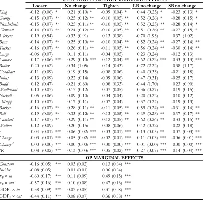
-King 0.27 (0.26) -0.83 (0.50) *** 3.49 (0.81) *** 3.39 (0.79) ***
George 0.12 (0.27) -1.10 (0.53) ** 4.00 (1.02) *** 3.99 (0.86) ***
Plenderleith 0.20 (0.28) -1.06 (0.56) * 4.00 (1.04) *** 4.01 (0.83) ***
Clementi 0.23 (0.30) -0.97 (0.55) * 3.92 (1.05) *** 3.90 (0.92) ***
Vickers 3.35 (11.7) 3.21 (20.5) -3.67 (23.5) -5.33 (15.5)
Bean -0.07 (0.27) -1.02 (0.48) ** 3.96 (0.91) *** 3.98 (0.70) ***
Tucker -0.28 (0.31) -1.06 (0.49) ** 4.31 (0.80) *** 4.29 (0.79) ***
Large 0.34 (0.43) -0.39 (0.54) 1.58 (1.28) 1.76 (1.52)
Lomax -0.62 (0.35) * -1.55 (0.53) *** 4.70 (1.41) *** 4.76 (1.43) ***
Buiter 4.07 (17.0) 3.32 (22.5) -3.60 (24.7) -5.49 (17.8)
Goodhart 0.92 (0.57) -0.41 (0.71) 2.78 (1.60) * 3.04 (1.72) *
Julius 0.68 (0.46) -0.63 (0.65) 3.51 (1.43) ** 3.56 (1.31) ***
Budd 1.27 (1.02) 0.26 (1.46) 0.51 (4.24) -3.36 (13.4)
Wadhwani 0.80 (0.50) -0.30 (0.59) 2.32 (1.69) 2.72 (1.25) **
Nickell 0.66 (0.37) * -0.26 (0.49) 1.61 (1.20) 1.49 (1.25)
Allsopp 0.72 (0.47) -0.29 (0.53) 1.99 (1.60) 2.79 (1.08) **
Barker -0.05 (0.27) -0.91 (0.46) ** 4.51 (0.81) *** 4.49 (0.67) ***
Bell 0.01 (0.37) -0.81 (0.50) 5.06 (1.17) *** 5.31 (1.14) ***
Lambert -0.33 (0.35) -1.21 (0.52) ** 4.75 (1.25) *** 4.76 (1.11) ***
Walton -0.02 (0.64) -0.89 (0.76) 3.25 (1.99) 3.22 (1.89) **
Change -0.19 (0.08) ** -0.24 (0.06) *** -0.31 (0.06) ***
Change2 0.01 (0.01) ** 0.01 (0.01) ** 0.02 (0.00) ***
|r - r◊| -0.03 (0.14)
r 0.21 (0.09) ** 0.32 (0.11) *** 0.36 (0.15) **
IR 0.87 (0.20) *** 0.79 (0.22) *** 0.75 (0.16) ***
Constant 0.68 (0.12) *** 0.60 (0.12) *** 0.76 (0.12) *** 0.73 (0.17) ***
Insider 0.40 (0.13) *** 0.43 (0.14) *** 0.42 (0.15) *** 0.34 (0.23) πF × in 2.68 (0.63) *** 2.89 (0.68) *** 2.28 (0.69) *** 2.69 (0.65) *** πF × out 3.04 (0.58) *** 3.17 (0.58) *** 3.01 (0.54) *** 2.56 (0.53) *** GDPF × in 1.59 (0.23) *** 1.68 (0.25) *** 1.57 (0.30) *** 1.70 (0.27) *** GDPF × out 1.32 (0.26) *** 1.34 (0.27) *** 1.34 (0.28) *** 1.94 (0.32) ***
µ 1.35 (0.18) *** 1.21 (0.17) *** 1.27 (0.18) *** 1.45 (0.17) ***
ρεu -0.34 (0.17) **
ρpanel 0.25 (0.09) ***
AIC BIC CAIC Max L
***/**/* denotes two-tailed significance at the 1%/5%/10% level respectively
Models in the above table are defined as follows:
Model 1 IOP model with fixed effects (FEs) only in selection equation
Model 2 IOP model with FEs in selection equation
Model 3 Correlated IOP model
Model 4 IOP with FEs in selection equation and one RE in short-run adjustment equation -1385.5 1572.9 ORDERED PARAMETERS -1604.9 SUMMARY STATISTICS -- -1474.8 1632.9 1659.9 Model 4
SPLITTING FUNCTION PARAMETERS
-1647.1
Model 1 Model 2 Model 3
-
--697.9
-723.9 -676.8
IDIOSYNCRATIC AND COMPOSITE ERROR CORRELATION
[image:21.595.123.502.95.641.2]1422.6 1610.0 1642.0 -695.3 1427.7 1615.1 Table 1.
cant values. Excluding all statistically insignificant members in each group, the average
(estimated) internal member’s NNRI is just over 4.04% compared to 3.73% for external
members. Moreover, when considering members whose estimates are statistically signifi
-cant, internal members exhibit much more consensus with a tighter range of (3.39,4.76)
compared to (2.72,5.31).
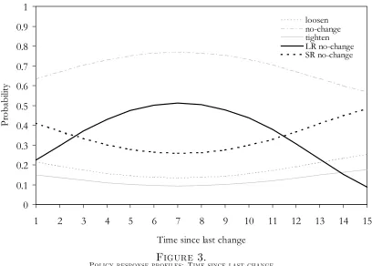
The (estimated) probability profiles with respect to time since last change are
pre-sented in Figure 3. These results suggest that overall, the probabilities of no-change
are not strongly affected by time since last policy change: rising slightly after the change,
peaking at around seven periods before dropping offas time passes. However, this total
disguises some significant counter-movements in the long-run and adjustment effects of
this variable. The pronounced n−shaped profile of no-change arising from the LR
equa-tion is consistent with a signalling argument: a recent change in rates has successfully
signalled a change in policy stance such that no further adjustment is necessary. This
effect is reinforced as time goes by (i.e., the probability of no-change increases). On the
other hand, the u−shaped profile of no-change probabilities from the SR equation, is
consistent with a (SR) stepping/smoothing argument: the NNRI has altered, such that a
recent policy change will trigger future ones. The greater the time since this last policy change, the greater is the likelihood of such further adjustments such that SR probabilities
of no-change decrease. It is the very nature of the model applied here, that allows us to
replicate two, superficially opposing aspects of monetary policy simultaneously.
There are significant random effects present in the short-run adjustment equation
of our preferred specification as indicated by the significance ofρpanel; further, likelihood
ratio tests reject equality of parameters of these Taylor-rule type variables across
member-type. As shown inTable 4,wefind that output gap effects are significant and signed as
expected: output below potential triggers a (significant) preference for rate decreases, and
vice versa. These effects appear to be stronger for external members: an interpretation of
thisfinding is that these members care relatively more about output. Finally, turning to
the inflation target deviations, we can see that this variable exerts a significantly positive
effect for both internal and external members: the further consensus inflation forecasts
are from target, the stronger is the preference for rate rises, and vice versa. However,
King -0.12 (0.06) * 0.21 (0.10) * -0.09 (0.04) * 0.44 (0.23) * -0.23 (0.13) *
George -0.15 (0.07) ** 0.25 (0.12) ** -0.10 (0.05) ** 0.52 (0.26) * -0.28 (0.15) *
Plenderleith -0.15 (0.07) ** 0.25 (0.11) ** -0.10 (0.05) ** 0.52 (0.25) ** -0.28 (0.14) *
Clementi -0.14 (0.07) ** 0.24 (0.12) ** -0.10 (0.05) ** 0.51 (0.26) ** -0.27 (0.15) *
Vickers 0.19 (0.54) -0.33 (0.91) 0.13 (0.38) -0.70 (1.93) 0.37 (1.02)
Bean -0.14 (0.07) ** 0.25 (0.10) ** -0.10 (0.04) ** 0.52 (0.24) ** -0.27 (0.14) **
Tucker -0.16 (0.07) ** 0.26 (0.11) ** -0.11 (0.05) ** 0.56 (0.24) ** -0.30 (0.14) **
Large -0.06 (0.07) 0.11 (0.11) -0.04 (0.05) 0.23 (0.24) -0.12 (0.13)
Lomax -0.17 (0.06) *** 0.29 (0.10) *** -0.12 (0.04) ** 0.62 (0.22) *** -0.33 (0.13) ***
Buiter 0.20 (0.62) -0.34 (1.05) 0.14 (0.43) -0.72 (2.22) 0.38 (1.17)
Goodhart -0.11 (0.09) 0.19 (0.15) -0.08 (0.06) 0.40 (0.33) -0.21 (0.18)
Julius -0.13 (0.09) 0.22 (0.14) -0.09 (0.06) 0.47 (0.31) -0.25 (0.17)
Budd 0.12 (0.47) -0.21 (0.80) 0.08 (0.33) -0.44 (1.70) 0.23 (0.90)
Wadhwani -0.10 (0.07) 0.17 (0.12) -0.07 (0.05) 0.36 (0.27) -0.19 (0.15)
Nickell -0.05 (0.06) 0.09 (0.10) -0.04 (0.04) 0.20 (0.22) -0.10 (0.12)
Allsopp -0.10 (0.07) 0.17 (0.11) -0.07 (0.04) 0.37 (0.24) -0.19 (0.13)
Barker -0.16 (0.07) ** 0.28 (0.11) ** -0.11 (0.05) ** 0.59 (0.24) ** -0.31 (0.14) **
Bell -0.19 (0.08) ** 0.33 (0.12) ** -0.13 (0.05) ** 0.69 (0.28) ** -0.37 (0.17) **
Lambert -0.17 (0.07) ** 0.29 (0.11) ** -0.12 (0.05) ** 0.62 (0.26) ** -0.33 (0.15) **
Walton -0.12 (0.09) 0.20 (0.15) -0.08 (0.06) 0.42 (0.32) -0.22 (0.18)
r 0.04 (0.01) *** -0.06 (0.02) *** 0.03 (0.01) *** -0.13 (0.05) ** 0.07 (0.03) **
Change -0.03 (0.01) *** 0.05 (0.02) *** -0.02 (0.01) *** 0.11 (0.03) *** -0.06 (0.01) ***
Change2 0.00 (0.00) *** 0.00 (0.00) *** 0.00 (0.00) *** -0.01 (0.00) *** 0.00 (0.00) ***
IR 0.08 (0.02) *** -0.13 (0.03) *** 0.05 (0.02) *** -0.27 (0.07) *** 0.14 (0.04) ***
Constant -0.16 (0.05) *** 0.03 (0.02) 0.13 (0.04) ***
Insider -0.08 (0.05) 0.01 (0.01) 0.06 (0.04) πF × in -0.60 (0.17) *** 0.11 (0.09) 0.49 (0.15) *** πF × out -0.57 (0.16) *** 0.10 (0.08) 0.47 (0.13) *** GDPF × in -0.38 (0.09) *** 0.07 (0.05) 0.31 (0.08) *** GDPF × out -0.44 (0.11) *** 0.08 (0.07) 0.36 (0.08) ***
***/**/* denotes two-tailed significance at the 1%/5%/10% level respectively
SPLITTING FUNCTION MARGINAL EFFECTS
OP MARGINAL EFFECTS
[image:23.595.108.523.191.598.2]SR no change Loosen No change Tighten LR no change
Table 2.
0 0.1 0.2 0.3 0.4 0.5 0.6 0.7 0.8 0.9 1
1 2 3 4 5 6 7 8 9 10 11 12 13 14 15
Time since last change
P
ro
b
ab
ili
ty
[image:24.595.114.522.101.393.2]loosen no-change tighten LR no-change SR no-change
Figure 3.
Policy response profiles: Time since last change
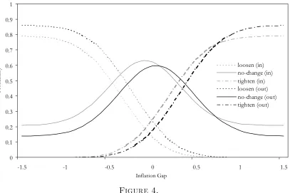
probability profiles for both cohorts is plotted below in Figure 4.
AsFigure 4illustrates, probabilities of no-change for both member groups peak when
consensus inflation forecasts tend to target rates. As the gap increases (decreases) a clear
shift towards a preference for a tightening (loosening) of policy is observed. However,
in terms of preferences for tightening when (forecast) inflation is too high, probabilities
for internal members are dominated by those for external members. Similarly, when the
gap is negative when (forecast) inflation is too low, external members have a stronger
preference for a loosening of policy, than their internal counterparts. Overall, it appears
that probabilities for no-change are uniformly dominated by internal members. This
finding is in line with Spencer (2006), whofinds that external members are more likely to
want to adjust rates.
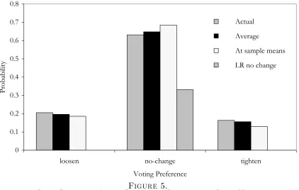
Finally, we undertake some model evaluation exercises. In Figure 5 we plot:
sam-ple proportions; average estimated probabilities; and probabilities evaluated at observed
sample covariate averages. For the latter the total probability of no-change is split into its
0 0.1 0.2 0.3 0.4 0.5 0.6 0.7 0.8 0.9 1
-1.5 -1 -0.5 0 0.5 1 1.5
Inflation Gap
Pr
o
b
ab
ilit
y loosen (in)
[image:25.595.118.525.107.378.2]no-change (in) tighten (in) loosen (out) no-change (out) tighten (out)
Figure 4.
Probability response profiles: Insiders and Outsiders
of no-change is dominated by its long-run component: a disaggregation not possible using
simple OP techniques, for example. This figure also shows that model closely mimics
observed sample proportions. We next consider the model’s predictive ability in terms of
contingency tables, based on the maximum probability rule (Table 3). Also presented
are those from a simple OP model (with the same specification inz). Our preferred model
(79% correct predictions) significantly outperforms its simpler OP counterpart (67%
cor-rect predictions). Note though, that in both models the bulk of the corcor-rect predictions
come from over-prediction of the heavily chosen “no-change” outcome. In ignoring the
underlying stochastic elements in the economic model and using the maximum
proba-bility rule, such models typically tend to over-predict the empirically most frequently
chosen outcome. Following Duncan and Weeks (1998) we also present a “simulated” hit
and miss table Table 4, where the preferred voting choice for each member is simulated
using re-sampling techniques with 1,000 independent random draws, and the resulting
independent hit and miss tables averaged over the R= 1,000 draws.
Here we now witness a reduction in correct predictions (to 57%), but a much more
0 0.1 0.2 0.3 0.4 0.5 0.6 0.7 0.8
loosen no-change tighten
Voting Preference
Probability
Actual
Average
At sample means
[image:26.595.104.526.114.382.2]LR no change
Figure 5.
Sample Proportions; Average Probabilities; Probabilities at Sample Means; and Long Run Probability of No Change
0 1 2 Total
0 59 (46) 136 (149) 0 (0) 195
Actual 1 28 (18) 544 (563) 27 (18) 599
2 1 (0) 118 (123) 36 (32) 155 Total 88 (86) 798 (798) 63 (65) 949
Predicted
Table 3.
Contingency table for fixed effects IOP Model 4 (OP Results in parentheses)
0 1 2 Total
0 73 105 17 195
Actual 1 95 422 83 599
2 18 88 49 155
Total 186 615 148 949
[image:26.595.140.484.591.686.2]Predicted
Table 4.
7
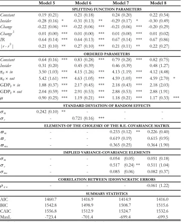
Sensitivty Analysis (Models 5-8)
For completeness, we also estimate the inertia and adjustment equations under various
assumptions of random effects (Models 5−8, Table 5). Specifically, we have: Model 5
- σ2
α 6= 0, σ
2
e = 0, σαe = 0 and ρεu = 0; Model 6 - σ
2
α = 0, σ
2
e 6= 0, σαe = 0 and ρεu = 0;
Model 7 - σ2
α 6= 0, σ
2
e 6= 0, σαe 6= 0 and ρεu = 0; and Model 8 - σ
2
α, σ
2
e, σαe and ρεu 6= 0.
Only weak evidence was found for the statistical presence of these additional variance
and covariance terms. The remaining specifications (in addition to the variance terms)
closely follow that of the fixed effects specifications (Model 2), although we now allow
for correlations across member-type in the inertia equation, by additionally including the
insider dummy.5
From this suit of models, the information criteria (BIC and CAIC) suggest a preference
for Model 6. Indeed, this specification is very close in spirit to that of Model 4 above.
Whilst the presence offixed effects is justified ona priori grounds, we note that the results
from Model 6 are ostensibly very similar to those of Model 4. That is, in the inertia
equation there is an−shaped profile in time since last change; the inflation report exerts
a positive influence on propensity to change probabilities; and the difference between the
prevailing interest rate and the NNRI also increases change probabilities. Finally, the
negative coefficient on the insider dummy suggests that insiders have a lower propensity
for change. We find that in line with Models 1-4, all parameters in the adjustment
equation are correctly signed (marginal effects available on request). However, while the
insider dummy is insignificant across all models, all interaction terms are significant at
the 1% level. This is consistent with the view that insiders and outsiders react differently
to changes in forecast inflation and output.
8
Conclusions
This paper attempts to empirically account for the empirical stylised facts of monetary
policy conducted by central banks whose primary objective is inflation targeting: those
of interest rate inertia, stepping and smoothing. This is undertaken by combining a
“long-run”, or propensity to change equation, with a “short-run”, or adjustment
Constant 0.19 (0.21) 0.21 (0.18) 0.24 (0.20) 0.22 (0.54)
Insider -0.28 (0.16) * -0.31 (0.13) ** -0.29 (0.17) * -0.30 (0.49)
Change -0.22 (0.06) *** -0.22 (0.06) *** -0.21 (0.06) *** -0.20 (0.29)
Change2 0.01 (0.00) *** 0.01 (0.00) *** 0.01 (0.00) *** 0.01 (0.02)
IR 0.64 (0.14) *** 0.64 (0.13) *** 0.67 (0.14) *** 0.67 (0.86)
|r - r◊| 0.21 (0.10) ** 0.27 (0.10) *** 0.21 (0.11) ** 0.22 (0.27)
Constant 0.64 (0.16) *** 0.83 (0.28) *** 0.79 (0.28) *** 0.82 (0.75)
Insider 0.31 (0.20) 0.45 (0.39) 0.46 (0.39) 0.48 (1.27) πF × in 3.50 (1.03) *** 4.15 (1.26) *** 4.13 (1.19) *** 4.12 (4.48) πF × out 5.42 (1.61) *** 4.63 (1.05) *** 4.59 (1.05) *** 4.59 (2.70) * GDPF × in 1.88 (0.37) *** 2.17 (0.45) *** 2.18 (0.43) *** 2.18 (2.03) GDPF × out 2.04 (0.59) *** 2.91 (0.53) *** 2.88 (0.53) *** 2.88 (1.91)
µ 0.90 (0.25) *** 1.19 (0.21) *** 1.18 (0.21) *** 1.17 (0.33) ***
σα 0.242 (0.10) **
σe 0.721 (0.16) ***
ϖα 0.233 (0.12) ** 0.226 (0.40)
ϖe 0.619 (0.19) 0.615 (0.95)
ϖαe 0.365 (0.25) 0.364 (1.90)
σα 0.054 (0.05) 0.051 (0.18)
σe 0.517 (0.24) ** 0.511 (1.04)
σαe 0.085 (0.06) 0.082 (0.37)
ρεu -0.061 (1.22)
AIC BIC CAIC MaxL
***/**/* denotes two-tailed significance at the 1%/5%/10% level respectively
Models in the above table are defined as follows:
Model 5 Inflated ordered probit with random effects in the selection equation only
Model 6 Inflated ordered probit with random effects in the OP equation only
Model 7 Inflated ordered probit with random effects in both equations
Model 8 Correlated inflated ordered probit with random effects in both equations
SUMMARY STATISTICS
CORRELATION BETWEEN IDIOSYNCRATIC ERRORS
-ELEMENTS OF THE CHOLESKY OF THE R.E. COVARIANCE MATRIX
- -- -1416.0 1515.6 1532.6 -699.5 1414.9 1508.7 1524.7 -699.4 1416.9 1498.9 1512.9 -701.4 1460.7 1542.8 1556.8 -723.4 -
-SPLITTING FUNCTION PARAMETERS
ORDERED PARAMETERS
STANDARD DEVIATION OF RANDOM EFFECTS
IMPLIED VARIANCE-COVARIANCE ELEMENTS
[image:28.595.127.507.135.592.2]
-Model 5 Model 6 Model 7 Model 8
Table 5.
tion. Importantly, we also allow for unobserved heterogeneity in both of these implicit
equations. This econometric modeling is undertaken within a discrete-choice outcome,
such that a new statistical model, the (Correlated) Inflated Ordered Probit, is proposed.
utilising the panel nature of our data, unobserved effects were conditioned in both of the
implicit underlying structural equations. Moreover, such a model explicitly takes into
account the large build-up of “no-change” observations witnessed in the monetary stance
of central banks worldwide.
The model was applied to the voting preferences of the Bank of England’s MPC members. The data appeared to be well-modelled by such an approach, and there is
evidence that external and internal members of the MPC react differently to the economic
environment. Finally, although there were some difficulties in finding appropriate proxies
for the inertia equation, the adjustment equation was well explained by primarily a
Taylor-rule type specification, where the Taylor (1993) variables, due to the lags involved in
References
Bean, C. (2004): Some Current Issues in UK Monetary Policy - Speech Given to the Institute of Economic Affairs in London on Wednesday 28th July 2004.
Belden, S. (1989): “Policy Preferences of FOMC Members as Revealed by Dissenting
Votes,”Journal of Money, Credit and Banking, 21(4), 432—441.
Bernhardsen, T.(2005): “The Neutral Real Interest Rate,” StaffMemo 2005/1, Norges
Bank.
Bhattacharjee, A., and S. Holly (2005): “Inflation Targeting, Committee Deci-sion Making and Uncertainty: The Case of the Bank of England’s MPC,” Cambridge
Working Papers in Economics 05/30, University of Cambridge.
Budd, A. (1998): “The Role and Operations of the Bank of England Monetary Policy
Committee,”Economic Journal, 108, 1783—1794.
Butler, J., and R. Moffitt (1982): “A Computationally Efficient Quadrature
Proce-dure for the One Factor Multinomial Probit Model,”Econometrica, 50.
Carare, A., and R. Tchaidze (2005): “The Use and Abuse of Taylor Rules: How
Precisely Can We Estimate Them?,” Discussion paper, International Monetary Fund.
Chappell, H. W. J., T. Havrilesky, and R. McGregor (1993): “Partisan
Mon-etary Policies: Presidential Influence Through the Power of Appointment,” Quarterly
Journal of Economics, 108(1), 185—218.
Clarida, R., J. Gali, and M. Gertler (2000): “Monetary Policy Rules and
Macro-economic Stability: Evidence and Some Theory,”Quarterly Journal of Economics, 115,
147—180.
Clerc, L., and T. Yates (1999): “Interest Rate Stepping: Some Puzzles and Facts,”
mimeo, Bank of England.
Davutyan, N., and W. Parke(1995): “The Operations of the Bank of England
1890-1908: A Dynamic Probit Approach,”Journal of Money, Credit and Banking, 27, 1099—
Dolado, J., and R. Maria-Dolores (2002): “Evaluating Changes in the Bank
of Spain’s Interest Rate Targets: An Alternative Approach Using Marked Point
Processes,”Oxford Bulletin of Economics and Statistics, 64, 159—182.
(2005): “Are Monetary Policy Reaction Functions Asymmetric? The Role of
Non-Linearity in the Phillips Curve,”European Economic Review, 49, 485—503.
Duncan, A., and M. Weeks (1998): “Simulating Transitions Using Discrete Choice
Models,”Proceedings of the American Statistical Association, 106, 151—156.
Eichengreen, B., M. Watson, and R. Grossman(1985): “Bank Rate Policy under
the Interwar Gold Standard: A Dynamic Probit Approach,” Economic Journal, 95,
725—745.
Eijffinger, S., E. Schaling, and W. Verhagen(1999): “A Theory of Interest Rate
Stepping: Inflation Tageting in a Dynamic Menu Cost Model,” Discussion paper 2168,
Centre for Economic Policy Research.
Eijffinger, S., and W. Verhagen (1999): “Should Monetary Policy Be Adjusted
Frequently?,” Discussion paper 2074, Centre for Economic Policy Research.
Engle, R., and C. Granger (1987): “Cointegration and Error-Correction:
Represen-tation, Estmation and Testing,”Econometrica, 55, 251—276.
Engle, R., and J. Russell (1997): “Forecasting the Frequency of Changes in Quoted
Foreign Exchange Prices with the Autoregressive Conditional Duration Model,”Journal
of Empirical Finance, 12, 187—212.
(1998): “Autoregressive Conditional Duration: A New Model for Irregularly
Spaced Transaction Data,” Econometrica, 66, 1127—1162.
Fry, M., D. Julius, L. Mahadeva, S. Roger,and G. Sterne(2000): “Key Issues in
the Choice on Monetary Policy,” inMonetary Policy Frameworks in a Global Context,
ed. by L. Mahadeva, and G. Stern. London: Routledge.
Gerlach-Kristen, P.(2004): “Is the MPC’s Voting Record Informative About Future
UK Monetary Policy?,”Scandinavian Journal of Economics, 106(2), 299—313.
Goodfriend, M. (1991): “Interest Rates and the Conduct of Monetary Policy,”
Carnegie-Rochester Series on Public Policy, 34, 7—30.
Goodhart, C.(1999): “Central Bankers and Uncertainty,” inProceedings of the British Academy: 1998 Lectures and Members. Oxford University Press.
Goodhart, C. A. E. (1996): “Why Do the Monetary Authorities Smooth Interest Rates?,” mimeo, London School of Economics Financial Markets Group.
Greene, W. (1994): “Accounting for Excess Zeros and Sample Selection in Poisson
and Negative Binomial Regression Models,” Working Paper EC-94-10, Stern School of
Business, New York University, Stern School of Business, New York University.
Greene, W. (2003): Econometric Analysis. Prentice Hall, New Jersey, USA,fifth edn.
Greene, W. (2004): “The Behaviour of the Maximum Likelihood Estimator of Limited
Dependent Variable Models in the Presence of Fixed Effects,” Econometrics Journal,
7(1), 98—119.
Hamilton, J., and O. Jorda (2002): “A Model of the Federal Funds Target Rate,”
Journal of Political Economy, 110, 1135—1167.
Harris, M., and X. Zhao (2004): “Modelling Tobacco Consumption with a
Zero-Inflated Ordered Probit Model,” Working Paper 14/04, Monash University, Department
of Econometrics and Business Statistics, Monash University, Australia.
Havrilesky, T., andJ. Gildea(1991): “The Policy Preferences of FOMC Members as
Revealed by Dissenting Votes: A Comment,” Journal of Money, Credit and Banking,
23(1), 130—138.
Havrilesky, T., and R. Schweitzer (1990): “A Theory of FOMC Dissent Voting
with Evidence from the Time Series,” inThe Political Economy of American Monetary