Approximations to the Normal Distribution Function and An Extended Table for the Mean Range of the Normal Variables

Approximations to the Normal

Distribution Function and An Extended

Table for the Mean Range of the Normal

Variables

Kiani, M and Panaretos, J and Psarakis, S and Saleem, M

JIRSS (2008)

Vol. 7, Nos. 1-2, pp 57-72

Approximations to the Normal Distribution

Function and An Extended Table for the Mean

Range of the Normal Variables

M. Kiani1, J. Panaretos2, S. Psarakis2, M. Saleem3

1

Department of Statistics, Athens University of Economics and Business & Payame-Noor University. (mk mehdi.kiani@yahoo.com)

2

Department of Statistics, Athens University of Economics and Business.

3

Department of Statistics, QUAID-i-AZAM University, Islamabad, Pakestan.

Abstract. This article presents a formula and a series for approx-imating the normal distribution function. Over the whole range of the normal variablez, the proposed formula has the greatest absolute error less than 6.5e₋09, and series has a very high accuracy. We examine the accuracy of our proposed formula and series for various values ofz’s. In the sense of accuracy, our formula and series are su-perior to other formulae and series available in the literature. Based on the proposed formula an extended table for the mean range of the normal variables is established.

1

Introduction

The normal distribution function (NDF) plays a central role in sta-tistical theory, where,

Φ(z) = √1

2π

Z z

−∞

e−t

2

2 dt, − ∞< z <+∞. (1)

The approximations for the NDF have been presented by Zelen and Severo (1946), Abramowitz and Stegun (1964), Hart (1966), Schucany and Gray (1968), Strecock (1968), Cody (1969), Badhe (1976), Ker-ridge and Cook (1976), Derenzo (1977), Hamaker (1978), Parsonson (1978), Heard (1979), Moran (1980), Lew (1981), Martynov (1981), Monahan (1981), Edgeman (1988), Pugh (1989), Vedder (1993), John-son, et al. (1994), Bagby (1995), Waissi and Rossin (1996), Bryc (2002), Marsaglia (2004), Shore (2004), Shore (2005), and several other authors.

In this paper, a new formula and a new series, for calculating the function Φ(z), are introduced. The advantages of the proposed approximations over the existing ones in literature are discussed. The new approximations to the Φ(z) are based on the error function,

erf(z). The integration region of the error function is (0, z) forz >0, or (0,₋z] forz_≤0 that is simpler than one of the Φ(z), such that,

erf(z) =

Z z 0

2

√

πe

−t2_{dt, − ∞< z <+∞, (2)}

Φ(z) = 1

2(1−erf(−z/

√

2)), _{− ∞}< z <+_∞. (3)

The mean range of the random variablesZ1, Z2, . . . , Znwith the

nor-mal distribution,E(R), forn= 2,(1)30 is tabulated by Montgomery (2005). The present paper sets out an extended table to E(R), for

n = 2,(1)100,(20)1020 where E(R) is computed according to the proposed formula to the NDF.

2

Formulae to Approximate the NDF

2.1 Existing Formulae

An approximation to Φ(z)₋0.5 with absolute error less than 3_×10−5

when z >0 is given by Bagby (1995),

Φ(z)₋0.5 _≃ 0.5_{1₋(1/30)[7 exp(₋z2/2) + 16 exp(₋z2(2₋√2)) +(7 +πz2/4) exp(₋z2)]_}0.5. (4) In this case, the approximation is obtained by using the polar integral based on [Φ(z)₋0.5]2.

A sigmoid approximation is indicated by

Φ(z) = 1/[1 + exp(

∞

X

k=0

akz2k+1)].

Based on this approximation, a simple formula with maximum abso-lute error 4.31_×10−5 _{forz∈[−8,+8] was introduced by Waissi and}

Rossin (1996),

Φ(z)_≃1/(1 + exp[₋√π(β1z5+β2z3+β3z)]), forz∈[−8,+8]. (5)

where β1 = −0.0004406, β2 = 0.0418198, β3 = 0.9000000. Bryc

(2002) presented a formula with maximum absolute error 1.9_×10−5_,

according to rational approximations to Mill’s ratio, 1₋Φ(z)_≃

z2_{+ 5.575192695z+ 12.77436324}

√

2πz3_{+ 14.38718147z}2_{+ 31.53531977z+ 2×12.77436324}e

−z2/2₍₆₎

This formula gives at least two significant digits precision for allz >0. Using the response modeling methodology, an approximation for the NDF, having greatest absolute error 2_×10−6 _{was suggested by}

Shore (2004). Later, Shore (2005) improved his proposed formula in Shore (2004) to the following formula with a maximum absolute error 6_×10−7 _{, such that,}

Φ(z)_≃[1 +g(₋z)₋g(₋z)]/2, for ₋9< z <9. (7) In this case,

g(z) = exp_{−log(2) exp_{[α/(λ/S1)][(1 +S1z)(λ/S1)−1] +S2z}}

where λ =₋0.61228883; S1 =−0.11105481; S2 = 0.44334159; α =

2.2 New Formula

As noted in the preceding section, the integration region to the func-tion erf is simpler than one of the NDF. Hence, the construction of the proposed formula is based on the error function. Replacing z by

−z/√2 in (2),

erf(₋z/√2) = _√2

π

Z ₋z/√2 0

e−t2_{dt, for − ∞< z <+∞. (8)}

Let,

I =

Z ₋z/√2 0

e−t2_{dt, for − ∞< z <+∞.(9)}

I2 =

Z ₋z/√2 0

Z ₋z/√2 0

e(−t21+t 2 2)dt

1dt2, for − ∞< z <+∞.(10)

The integrand of polar integral is less variable than the original one; thus, using the definition of trigonometric functionst1 =rcos(β) and

t2 =rsin(β), forz≤0 equation (10) is transformed to

I2 =

Z π/4 0

Z ₋z/(cos(β)√2)

0 re

−r2_drdβ

+

Z π/2

π/4

Z ₋z/(sin(β)√2)

0 re

−r2_drdβ

=

Z π/4 0

(1₋e−(z/(cos(β)√2))2_)dβ.

Denote,

ω(β) = (1/(cos(β)√2))2). (11) Transformingω(β) in polar coordinates toω(z) in rectangular coor-dinates, we get,

ω(z) = ln 1₋ 4

π(

Z ₋z/√2

0 e

−t2_dt)2

!

/₋z2. (12)

ThereforeI2=Rπ/4

0 (1−e−(z)

2

ω(z)_{)dβ, and,}

I =

r

π

4(1−e−

(z)2_ω(z)

), for z_≤0. (13)

In the sequel, combining (8), (9), and (13), forz_≤0, we have

Now, equation (10) is evaluated under the assumption that z > 0. When 0 > t1 ≥ t2 ≥ −z/√2 then π ≤ β ≤ 5π/4 and 0 < r ≤

−z/(cos(β)√2), whereas, when 0 > t1 ≥t2 ≥ −z/√2 then 5π/4 <

β _≤3π/2 and 0< r_{≤ −}z/(sin(β)√2). As a result, the calculations on I2, on behalf of z >0, yield andI =₋[π(₋e−(z)2ω(z)_{+ 1)/4]}1/2

erf(₋z/√2) =₋2I/√π, for z >0. (15) Define,

sign(₋z) =

(

−1 if z >0 1 if z_≤0

Because of (14) and (15), theerf(₋z/√2) over the whole range ofz

will be

erf(₋z/√2) =sign(₋z)

q

1₋e−z2ω(z)_{, for −∞< z <+∞. (16)}

Combining equations (3) and (16) we will have,

Φ(z) = 1

2(1−sign(−z)

q

1₋e−z2ω(z)_{), for − ∞< z <+∞ (17)}

The function ω(z) is approximated by ωA(z), such that,

ωA(z) = (18)

                        

−6.62e−6|z|5

+ 4.4166e−4z4

−1.31e−5|z|3

−9.56/17e−3z2

−4.8e−7|z|+/.636619771 0≤ |z|<1.05

−1.401663e−4|z|5

+ 1.150811e−3z4

−1.582555e

−3|z|3

−7.76126e−3z2

−1.0608e−3|z|+ 0.6368751 1.05≤ |z|<2.29

5.8716e−5|z|5

−1.221684e−3z4

+ 9.841663e−3|z|3

−3.55101e−2z2

+ 3.29203e−2|z|+ 0.62010268 2.29≤ |z|<8

0.5 8≤ |z|.

Substituting theωA(z) in equations (16) and (17), then the

approxi-mationserfA(−z/√2) and ΦA(z) is derived. Equivalently, for eachz,

we haveerf(z)_≃erfA(z) = 1−2ΦA(−z/

√

2). It is highly appropri-ate, for_|z_{| ≥}5.5, the functions erfA(z) and ΦA(z) to be constructed

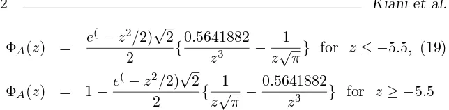
by applying rational chebyshev approximations. In this case, the ra-tional function of degreelin the numerator andmin the denominator is approximately defined byRlm(1/z2)≃0.5641882. As a result,

ΦA(z) =

1

2(1−sign(−z)

q

1₋e₋z2_ω

ΦA(z) =

e(₋z2/2)√2 2 {

0.5641882

z3 −

1

z√π} for z≤ −5.5, (19)

ΦA(z) = 1−

e(₋z2/2)√2 2 {

1

z√π −

0.5641882

z3 } for z≥ −5.5

Numerical experiments have shown that, for allz, the greatest abso-lute error to ΦA(z) anderfA(z) is less than 6.5×10−9 and 1.6×10−8,

respectively.

Table 1 is established to compare the performance of the studied and the proposed formulae.

Table 1. Absolute error of the formulae to approximate the NDF.

Formula Z=-30 Z=-10 Z=-6.5 Z=-5.5 Z=-4.5 (4) 4.9E-198 7.6E-24 1.6E-13 5.5E-10 1.2E-07 (5) 1.0E+00 6.3E-06 3.5E-10 1.6E-08 3.6E-07 (6) 1.8E-200 3.6E-26 1.6E-13 6.7E-11 9.6E-09 (7) i i 3.5E-11 8.3E-09 2.7E-07 (19) 1.8E-203 2.2E-27 6.2E-14 5.5E-11 1.5E-09 Formula Z=-3.5 Z=-2.5 Z=-1.5 Z=-0.5 Z=0

(4) 2.3E-06 1.1E-05 1.9E-05 2.8E-05 0.0E+00 (5) 3.4E-06 3.4E-05 1.6E-05 2.6E-05 0.0E+00 (6) 4.6E-07 6.5E-06 1.9E-05 1.6E-06 0.0E+00 (7) 5.2E-07 3.1E-07 7.6E-08 5.7E-08 0.0E+00 (19) 3.3E-10 1.1E-09 3.0E-09 2.1E-09 0.0E+00

”i” indicates a complex number.

This table shows the absolute errors involved in the formulae, such that approximation (19) has minimum absolute error over the wide range of z. The formulae (5) and (7) fail to approximate the NDF for absolute amounts of largez’s.

3

Series to Approximate the NDF

In the sequel, series expansions to approximate the NDF will be rep-resented. In addition, a new series with very high accuracy is given.

3.1 Existing Series

com-plementary error function,erf c(x), where,

erf c(x) = 1₋erf(x) = _√2

π

Z _∞

x

e−t2_dt.

The presented approximations are,

erf(x) _≃ xRlm(x2) =x n

X

j=0

pjx2j/ n

X

j=0

qjx2j, |x| ≤0.5,

erf c(x) _≃ e−x2_R

lm(x2)

= e−x2

n

X

j=0

pjxj/ n

X

j=0

qjxj, 0.46875≤x≤4.0 (20)

erf c(x) _≃ e−

x2 x { 1 √ π + 1

x2Rlm(1/x 2₎

}

= e−

x2 x { 1 √ π + 1 x2 n X j=0

pjx−2j/ n

X

j=0

qjx−2j}, x≥4.0.

where, the coefficientspj and qj are tabulated for various value nin

the paper of Cody (1969). The maximum relative errors, for these approximations, ranging down to between 6_×10−19 _{and 6×10}−20

for all z.

Kerridge and Cook (1976) present a convergent Taylor expansion for computing Φ0(z), where Φ0(z) = Φ(z)−0.5 and,

Φ0(z) = Z z

0

1

√

2πe

f rac−t22_dt

≃ √1

2πze

−z 2 8 +∞ X n=0 1

2n+ 1θ2n(z/2), − ∞< z <+∞.(21) In this series, θn(z) = znHn(z)/n!, for n = 0,1,2, . . ., and Hn(z)

implies thenth Hermite polynomial, such thatH0(z) = 1,H1(z) =z,

and Hn+1(z) = zHn(z)−nHn−1(z) for n = 1,2, . . .. They suggest

some advantages for usingθn(z) overHn(z), such thatθn(z) are easier

to handle numerically and relatively small for largen,

θ0(z) = 1; θ1(z) =z2; θn+1(z) =

z2[θn(z)−θn−1(z)]

n+ 1 , forn= 1,2, . . . Recently, Marsaglia (2004) provided the approximation bellow,

Φ(z)_≃0.5 + (2π)−1/2_e−z2/2 _z+z

3

3 +

z5

3.5+

z7

3.5.7 +

z9

3.5.7.9+· · ·

!

.

Marsaglia’s series based on the Taylor expansion about zero for func-tion B(z),

B(z) =

Z z 0

e−t2/2_dte−z2/2_≃z+z

3

3 +

z5

3.5+

z7

3.5.7+· · · He provided the following C function, using C compiler libraries, for the computation of Φ(z),

double Phi(double z)

{Long double=z,t=0,b=z,q=z*z,i=1; while(s!=t)s=(t=s)+(b*=q/(i+=2));

return 0.5+s*exp(-0.5*q-0.91893853320467274178L);}.

The accuracy of the proposed series by Kerridge and Cook (1976) and Marsaglia (2004) will be discussed, where the accuracy of these series rely on the terms used of series and the digits predefined for computing the approximations.

3.2 New Series

The function Φ(z) can be numerically approximated, utilizing the Taylor expansion toe−t2_,

e−t2 _≃e−c2

+∞

X

k=0

uk(c)

k! (t−c)

k_{, for}

− ∞< t <+_∞ (23)

where, c=t+α for 0< α_≤1, and,

u0(c) = 1; u1(c) =−2c;

uk(c) =−2(k−1)uk−2(c) + (−2c)uk−1(c), for k≥2.

Integrating on (23), with respect to tfrom 0 to₋z/√2,

Ierf =

Z ₋z/√2 0

e−t2_dt≃I

Aerf

= sign(₋z)

B+1 X

i=1

e−c2i

n→+∞

X

k+1

u(i,k)(ci)

k! (Ai+1−ci)

k_{, (24)}

where, B = round(_|z_|/√2), ci = Ai = (i−1)×round(|z|/B

√

2)),

AB+2 =|z|/√2,u(i,1)= 1,u(i,2)=−2ci,u(i,k) =−2[(k−2)u(i,k−2)+

ciu(i,k−1)], for i = 1,2, . . . , B+ 1 and k ≥ 3. Excepti-onally, B is

To avoid the calculation of equation (24) for large value B, inte-grating on (23) with respect totfrom ₋z/√2 to _±∞, let us define

Ierf e =

Z _∞

−z/√2

e−t2_dt≃I

Aerf

= sign(₋z)

m→+∞

X

i=1

e−c2i

n→+∞

X

k+1

u(i,k)(ci)

k! (Ai−ci)

k_{, (25)}

In this case, Ai = |z|/√2, A2 = round(|z|/√2) + 1, Ai+1 = Ai+ 1

fori_≥3, andci =Ai+1 fori≥1. Applying (24) and (25), the error

function and the complementary error function are approximated by

erf(₋z/√2) _≃ 2IAref/√π, (26)

erf(₋z/√2) _≃ 2IAref e/√π, (27)

As a consequence, corresponding to Φ(z) = 0.5_×erf c(₋z/√2) for

z_≤0 and Φ(z) = 1 + 0.5_×erf c(₋z/√2) forz >0, we will have the following approximation with very high precision,

Φ(z) _≃ 1 2

{√π₋2IAerf}

√

π for |z| ≤4,

Φ(z) _≃ IAerf e/√π for z≤ −4, (28)

Φ(z) _≃ 1 +IAerf e/√π for z≤ −4,

On behalf of _|z_{| ≤} 4, this approximation is accurate with at least 60 significant digits accuracy, when n_≥ 100 in (24). The digits for computing (28) is held equal or greater than 65 to achieve at least 60 significant digits accuracy for 0 _{≤ |}z_{| ≤} 70. Furthermore, the approximation (28) relies on the value m in series (25). Numerical experiments show, when m _≥ 10 for 4 _{≤ |}z_{| ≤} 45 and m _≥ 2 for 45_{≤ |}z_{| ≤} 70, the approximation (28) gives the desired accuracy, in at least 60 significant digits.

Generally, in practice, for 0 _{≤ |}z_{| ≤} 70, the approximation (28) has in at least 60 significant digits accuracy, whereas in theory arbi-trary accuracy can be achieved for all z. For example, according to the approximations (21), (22) and (28), applying Maple or C compiler libraries, we have,

Φ(₋70) = 0.54230396093013993286757866708

This means (28) is accurate in at least 60 significant digits. The calculations of Φ(₋70) are based on expansion truncated at 3309, about 13600, and 252 terms and Digits equated to 1127, about 3000, and 64 for series (21), (22), and (28), respectively.

The small terms, m and n, and small digits for computing are good properties for (28), such that the speed of calculation is too fast for either small or large z, 0 _{≤ |}z_{| ≤} 70. For very large value

z i.e., _|z_| > 70, if the significant digits accuracy is only important and the speed is not, then the approximation (28) is proposed, such that we holdm= 2, Digits:=70 and only increasen. Otherwise, the approximation (20) is proposed, where the speed of the calculation for this approximation is very fast and its accuracy is between 18 and 20 significant digits. Corresponding to numerical experiments, the number of terms, n, for a specific level of accuracy is almost a linear function of z. For example, for z = ₋600 the approximation (28) is truncated at n= 1080 terms, where

Φ(₋600) = 0.6546588205807692852105927713888 10878211941283185317721116943e₋78176.

We expect this approximation to be accurate, since larger terms to compute (28),n >1080, gives the same approximation for Φ(₋600), possessing 60 significant digits. Series (20) and formulae (6) and (19) approximate Φ(₋600) having 20, 3, and 10 significant digits accuracy, respectively. It is not easy to calculate Φ(₋600) according to series (21) and (22), because of the convergence of these series suffer from difficulties with very large terms required.

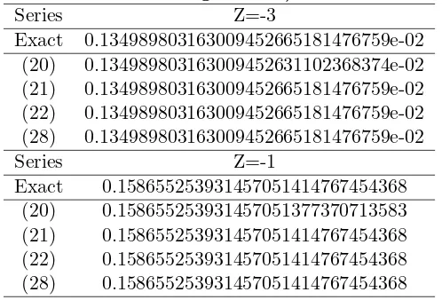
Table 2. Series to approximate the NDF, (160 terms and Digits:=200).

Series Z=-18

Exact 0.974094891893715048259189518997e-72 (20) 0.974094891893715048708181934747e-72 (21) 0.226820907630354110107306715331e-38 (22) 0.499999999999757093038012396287e-00 (28) 0.974094891893715048259189518997e-72 Series Z=-9

Exact 0.112858840595384064773550207597e-18 (20) 0.112858840595384064738093247631e-18 (21) 0.112858840595384064773550207597e-18 (22) 0.989596251047682032099597869127e-08 (28) 0.112858840595384064773550207597e-18

Table 2 (continued). Series to approximate the NDF, (160 terms and Digits:=200).

Series Z=-3

Exact 0.134989803163009452665181476759e-02 (20) 0.134989803163009452631102368374e-02 (21) 0.134989803163009452665181476759e-02 (22) 0.134989803163009452665181476759e-02 (28) 0.134989803163009452665181476759e-02 Series Z=-1

Exact 0.158655253931457051414767454368 (20) 0.158655253931457051377370713583 (21) 0.158655253931457051414767454368 (22) 0.158655253931457051414767454368 (28) 0.158655253931457051414767454368

Table 2 shows, under the conditions as mentioned, the series (21) and (22) are accurate, for small z’s, and series (20) is accurate with 18 to 20 significant digits for wide range ofz. Furthermore, this table shows series (28) is accurate in at least 30 significant digits for either small or large z’s.

accuracy accomplished of this approximation is constrained on 18 to 21 significant digits. Therefore the proposed series seems to be superior in at least these aspects. Statistical softwares (for example Matlab, S-plus and MS Excel) compute the Φ(z), for example Φ(₋1), with different significant digits. To overcome this problem, the new series is proposed to be used on the statistical packages, because of its advantages.

4

The Mean Range for Normal Distribution

To approximate the mean range of the normal variables, correspond-ing to equation (1), define the random variableZi’s, fori= 1,2, . . . , n.

Define, also, the range of order statistics Z₍₁₎, Z₍₂₎, . . . , Z_(n) by R =

Z_(n)−Z₍₁₎, and its mean by d2 i.e. E(R) =d2. Under these

condi-tions, the probability density function toR is

ϕR(r) =

Z +_∞

−∞

n(n₋1)[Φ(r+z)₋Φ(z)]n−2_{ϕ(z)ϕ(r+z)dz, r ≥0.}

where, the ϕ(z) denotes the normal density function. The evalu-ation to the mean range of the random variables with normal distri-bution is given by Johnson, et al. (1994), where,

E(R) =

Z +_∞

−∞

{1₋(F(z))n₋(1₋F(z))n_}dz.

To construct an extended table for d2 the Φ(z) is evaluated by the

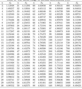
proposed formula (19) with maximum absolute error 6.5e-09. How-ever, although, the considered series are much more accurate than the formulae, but it is no possible or at least very difficult to evaluate the E(R), by using these series. Table 3 exhibits the mean range of the normal variablesZi for various values n= 2(1)100, 120(20)1020.

Table 3. The mean range of normal distribution (d2).

n d2 n d2 n d2 n d2 n d2

2 1.12838 31 4.11293 60 4.63856 89 4.93131 460 6.02251 3 1.69257 32 4.13934 61 4.65112 90 4.93940 480 6.04853 4 2.05875 33 4.16482 62 4.66346 91 4.94739 500 6.07340 5 2.32593 34 4.18943 63 4.67557 92 4.95529 520 6.09721 6 2.53441 35 4.21322 64 4.68747 93 4.96309 540 6.12004 7 2.70436 36 4.23625 65 4.69916 94 4.97079 560 6.14198 8 2.84720 37 4.25855 66 4.71065 95 4.97841 580 6.16308 9 2.97003 38 4.28018 67 4.72194 96 4.98593 600 6.18340 10 3.07751 39 4.30117 68 4.73305 97 4.99337 620 6.20301 11 3.17287 40 4.32155 69 4.74397 98 5.00073 640 6.22194 12 3.25846 41 4.34136 70 4.75472 99 5.00800 660 6.24023 13 3.33598 42 4.36063 71 4.76529 100 5.01519 680 6.25794 14 3.40676 43 4.37938 72 4.77570 120 5.14417 700 6.27509 15 3.47183 44 4.39764 73 4.78595 140 5.25118 720 6.29172 16 3.53198 45 4.41544 74 4.79604 160 5.34243 740 6.30786 17 3.58788 46 4.43279 75 4.80598 180 5.42186 760 6.32353 18 3.64006 47 4.44972 76 4.81578 200 5.49208 780 6.33876 19 3.68896 48 4.46624 77 4.82543 220 5.55497 800 6.35358 20 3.73495 49 4.48238 78 4.83493 240 5.61185 820 6.36800 21 3.77834 50 4.49815 79 4.84431 260 5.66375 840 6.38205 22 3.81938 51 4.51356 80 4.85355 280 5.71144 860 6.39573 23 3.85832 52 4.52864 81 4.86266 300 5.75553 880 6.40908 24 3.89535 53 4.54339 82 4.87165 320 5.79652 900 6.42211 25 3.93063 54 4.55783 83 4.88051 340 5.83480 920 6.43483 26 3.96432 55 4.57197 84 4.88926 360 5.87069 940 6.44725 27 3.99654 56 4.58582 85 4.89789 380 5.90446 960 6.45939 28 4.02741 57 4.59939 86 4.90641 400 5.93636 980 6.47126 29 4.05704 58 4.61270 87 4.91481 420 5.96655 1000 6.48287 30 4.08552 59 4.62575 88 4.92311 440 5.99522 1020 6.49423

5

Conclusion

New methods for the approximation of the normal distribution func-tion have been introduced. The accuracy and the speed of the cal-culations are advantages of the proposed methods over the some ex-isting methods. An extended table for the mean range of the normal variables has been constructed.

References

Badhe, S. K. (1976), New approximation of the normal distribution function. Communications in Statistics-Simulation and Com-putation, 5, 173-176.

Bagby, R. J. (1995), Calculating normal probabilities. The Ameri-can mathematical monthly. 102, 46-49.

Bryc, W. (2002), A uniform approximation to the right normal tail integral. Applied Mathematics and Computation, 127, 365-374.

Cody, W. J. (1969), Rational Chebyshev approximations for the error function. Mathematics of Computation, 23(107), 631-637.

Derenzo, S. E. (1977), Approximations for hand calculators using small integral coefficients. Mathematics of Computation, 31, 214-225.

Divgi, D. R. (1979), Calculation of univariate and bivariate normal probability function. The Annals of Statistics,7(4), 903-910. Edgeman, R. L. (1988), Normal distribution probabilities and

quan-tiles without tables. Mathematics of Computer Education, 22, 95-99.

Hamaker, H. (1978), Approximating the cumulative normal distri-bution and its inverse. Applied Statistics,27, 76-77.

Hart, R. G. (1966), A close approximation related to the error func-tion. Mathematics of Computation,20, and 600-602.

Heard, T. J. (1979), Approximation to the normal distribution func-tion. Mathematical Gazette, 63, 39-40.

Johnson, N. l., Kotz, S., and Balakrishnan, N. (1994), Continuous Univariate Distributions. 2nd edition. New York: Wiley. Kerridge, D. F. and Cook, G. W. (1976), Yet another series for the

normal integral. Biometrika, 63, 401-403.

Marsaglia, G. (2004), Evaluating the normal distribution. Journal of Statistical Software,11(4), 1-11.

Martynov, G. V. (1981), Evaluation of the normal distribution func-tion. Journal of Soviet Mathematics,17, 1857-1876.

Monahan, J. F. (1981), Approximation the log of the normal cu-mulative. Computer Science and Statistic: Proceeding of the Thirteenth Symposium on the Interface W. F. Eddy (editor), 304-307, New York: Springer-Verlag.

Moran, P. A. P. (1980), Calculation of the normal distribution func-tion. Biometrika,67, 675-676.

Montgomery, D. C. (2005), Introduction to Statistical Quality Con-trol. 5th edition. New York: John Wiley.

Parsonson, S. L. (1978), An approximation to the normal distribu-tion funcdistribu-tion. Mathematical Gazette, 62, 118-121.

Pugh, G. A. (1989), Computing with Gaussian Distribution: A Sur-vey of Algorithms. ASQC Technical Conference Transactions,

46, 496-501.

Schucany, W. R. and Gray, H. L. (1968), A new approximation related to the error function. Mathematics of Computation,

22, 201-202.

Shore, H. (2004), Response modeling methodology (RMM)-current statistical distributions, transformations and approximations as special cases of RMM. Communications in Statistics-Theory and Methods, 33(7), 1491-1510.

Shore, H. (2005), Accurate RMM-based approximations for the CDF of the normal distribution. Communications in Statistics-Theory and Methods, 34, 507-513.

Strecock, A. J. (1968), On the calculation of the inverse of the error function. Mathematics of Computation,22, 144-58.

Waissi, G. and Rossin, D. F. (1996), A Sigmoid approximation to the standard normal integral. Applied Mathematics and Com-putation, 77, 91-95.