Applying Linear Controls to Chaotic Continuous Dynamical Systems

http://dx.doi.org/10.4236/ojapps.2016.63015

Applying Linear Controls to Chaotic

Continuous Dynamical Systems

James Braselton, Yan Wu

Department of Mathematical Sciences, Georgia Southern University, Statesboro, GA, USA

Received 18 January 2016; accepted 13 March 2016; published 16 March 2016

Copyright © 2016 by authors and Scientific Research Publishing Inc.

This work is licensed under the Creative Commons Attribution International License (CC BY). http://creativecommons.org/licenses/by/4.0/

Abstract

In this case-study, we examine the effects of linear control on continuous dynamical systems that exhibit chaotic behavior using the symbolic computer algebra system Mathematica. Stabilizing (or controlling) higher-dimensional chaotic dynamical systems is generally a difficult problem,

Mu-sielak and MuMu-sielak, [1]. We numerically illustrate that sometimes elementary approaches can

yield the desired numerical results with two different continuous higher order dynamical systems that exhibit chaotic behavior, the Lorenz equations and the Rössler attractor.

Keywords

Chaotic Dynamical System, Lorenz Equations, Rössler Attractor, Chaos, Hyperchaos, Control, Stability, Routh-Hurwitz Theorem, Characteristic Polynomial

1. Introduction

We begin with an autonomous continuous dynamical system

d d

x

t

=

F x

( )

, where

1 2

n x

x

x       =_{ }     x

 and

( )

(

)

(

)

(

)

1 1 2 2 1 2

1 2

, , , , , ,

, , ,

n

n

n n

f x x x

f x x x

f x x x

 

 

 

=  

 

 

 

F x

  



We use the notation that *

(

x x₁, ₂, ,xn

)

∗ ∗ ∗

= 

x is a rest point, or equilibrium point of dx dt=F x

( )

, if

( )

* =

0

F x .

Under some parameter values or initial conditions, the system dx dt=F x

( )

exhibits chaos or hyperchaos. Refer to Yu et al., [2], for a discussion regarding the differences between chaos and hyperchaos.

Control theory attempts to find a controller to apply to the dynamical system that stabilizes the system and eliminates the chaos or hyperchaos. In the context of the autonomous dynamical system dx dt=F x

( )

, the investigator searches for a function G

( )

t,x so that dx dt=F x

( )

−G

( )

t,x does not exhibit chaos or hyperchaos for the given parameter values and initial conditions that the original system, dx dt=F x

( )

exhibits using those parameter values and initial conditions.

The focus of this paper is to illustrate an automated technique to find a linear control (G

( )

t,x ) of a continuous dynamical system that exhibits chaos or hyperchaos. In subsequent studies, we will focus both on the controller design, conditions when a chaotic system is stabilized, and the physical interpretation of the controller for specific dynamical systems.

2. Background

Li and Li, [3], provide examples of several approaches to controlling the chaotic three dimensional Chen-Lee system in their paper and illustrate how different multiple control techniques stabilize the system in their case study. To briefly summarize their results, Li and Li, [3], provide several approaches to control and provide synchronization of the chaotic Chen-Lee System,

d d

d d

1

d d .

3

X t ZY aX Y t XZ bY

Z t XY cZ = − +

= +

= +

(1)

at the origin, E₀=

(

0, 0, 0

)

. In their case study they use three feedback controls that are summarized as follows. (1) Linear Feedback Control. Linear −k X₁ , −k Y₂ and −k Z₃ terms are included in the x, y, and z

equations of system (1). The ki's are feedback coefficients. (2) Speed Feedback Control. A single control of the form

(

)

(

)

1 1 2

k −YZ+aX−k x +k XZ+bY

is incorporated into the x-equation of system (1). k₁ and k₂ are the speed feedback coefficients (see [4]). (3) Doubly-Periodic Function Feedback Control. The control in the X-equation is +k₁cn

(

X m₁,

)

and in the Z-equation is +k₃cn

(

Z m₁,

)

. The functions +k₁cn

(

X m₁,

)

and +k₃cn

(

Z m₁,

)

are the doubly-periodic functions where k₁ and k₃ are speed feedback coefficients and 0< <m 1 is the modulus of the Jacobi elliptic function. Refer to Li and Li, [3], for details.

The form of the design used to attempt to control a given system can be motivated by many factors. In general, controlling nonlinear high-dimensional chaotic dynamical systems can be a formidable problem, Musielak and Musielak, [1]. Viera and Lichtenberg, [5], illustrate several examples of controlling chaos using a nonlinear feedback with delay. On the other hand, Tan et al., [4], develop a controller using a backstopping design.

In this paper, we demonstrate a sequence of algorithms that may be used to find a linear control for a high- dimensional non-linear dynamical system that exhibits chaos or hyperchaos under certain conditions. We show that a basic linear control of the form −k x

(

−x*

)

, where k>0, can often be used to stabilize high-dimen-

sional non-linear chaotic dynamical systems provided that the underlying parameter values are known a priori. We use a computer algebra system like Mathematica or Maple to implement the procedure to find the simplest linear control, when possible. In this paper, we use Mathematica. The technique is described next.

(1) Begin with an autonomous continuous dynamical system, dx dt=F x

( )

, x

( )

t₀ = x₀.

(2) Assume that the appropriate parameter values and initial conditions are known and the system exhibits chaos or hyperchaos at an equilibrium point *

(3) Based on the known parameter values investigate a proportional controllerl of the form −k x

(

−x*

)

,

> k 0.

(4) If it is possible to find a proportional controller using the given constraints, the problem is solved. (a) Linearize the controlled system dx dt=F x

( )

−k x

(

−x*

)

at *

x .

(b) Compute the Jacobian, J x

( )

* , of the controlled system. To determine the maximum value of the real part

of the eigenvalues of J x

( )

* , try the following approaches that are well-suited to computer arithmetic.

(i) Obtain bounds on the real part of k using the Routh-Hurwitz theorem so that the maximum value of the real part of all eigenvalues of J x

( )

* are negative, if possible.

or

(ii) Compute the eigenvalues of J x

( )

* and then determine conditions on k so that the maximum value of

the real part of all eigenvalue is negative, if possible. Remark: Our simulations indicate that this yields better results than the Routh-Hurwitz theorem when the maximum value of the real part of the eigenvalues is close to 0.

(A) Given k, compute the eigenvalues of J x

( )

* by computing the zeros of the characteristic polynomial

of

( )

*

J x , p

( )

λ .

(B) Find the real part of all zeros of p

( )

λ .

(C) Find conditions on k so that the maximum value of the real part of all zeros of p

( )

λ is negative, if possible.

(5) Underlying Strategy: The “best” control is the simplest one. Thus, we start by searching for the simplest linear control possible.

For our case-studies we choose to numerically illustrate the techniques on versions of the Lorenz equations

and Rössler attractors because they are well studied and because of their broad use in applications. Of course, a similar analysis can be carried out with many other high-dimensional dynamical systems that exhibit chaotic behavior, which we hope to do in future studies where we will focus on the underlying physical interpretation of the control.

3. The Lorenz Equations

The Lorenz system is a three-dimensional continuous nonlinear dynamical system,

(

)

d d

d d

d d ,

X t Y X

Y t XZ RX Y

Z t XY bZ

σ

= −

= − + −

= −

(2)

that has numerous applications in areas such as simple models of lasers, thermosyphons, and some chemical reactions.

Parameter

σ

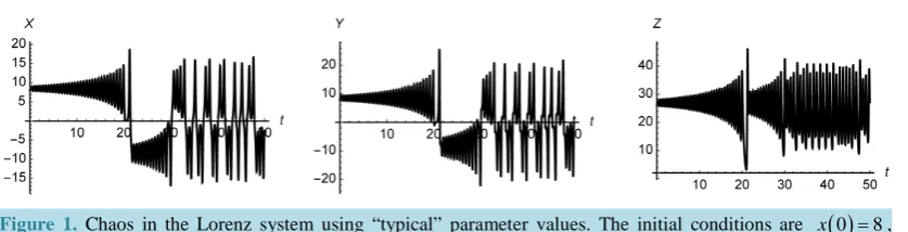
(sometimes replaced by P) is known as the Prandtl number, and is usually fixed to be 10 in many studies. b is the Biot number, fixed to be 8/3. R is the Raleigh number, which is typically taken to be greater than 28. With these parameter values, the Lorenz system, (2), exhibits chaos for a wide range of initial conditions.

For example, Figure 1 illustrates chaos in the Lorenz system using

σ

=10, =28, b=8 3 and the initial conditions X

( )

0 =8, Y

( )

0 =8, and Z

( )

0 =26. For these parameter values the Lorenz system has three

equilibrium points

1 2 0

8.48528 8.48528 27 8.48528 8.48528 27

0 0 0

X Y Z

E

E

E

[image:4.595.107.526.81.188.2]

Figure 1. Chaos in the Lorenz system using “typical” parameter values. The initial conditions are x

( )

0 =8,

( )

0 8

y = , and z

( )

0 =26.

The Jacobian of system (2) evaluated at each equilibrium point has the following eigenvalues

( )

( )

1,2,3 1,2

0

13.8546, 0.0939556 10.1945

22.8277,11.8277, 2.66667, E i E λ − ± − − J J

which shows that all three equilibrium points are unstable.

Using the described algorithm to try to find a control for an unstable equilibrium point, we choose an equilibrium point and search for the simplest control possible to stabilize it. To illustrate the concept, we choose

(

)

*

1 8.48528,8.48528, 27

E

= =

X . With this notation, X*=8.48528, Y*=8.48528, and Z*=27.

3.1. X-Control

We attempt to find the simplest control possible so search for an initial control of the form −k X

(

−X*

)

,

(

)

(

*

)

d d

d d

d d .

X t Y X k X X

Y t XZ RX Y

Z t XY bZ

σ

= − − −

= − + −

= −

(3)

Evaluated at * 1 E =

X , the Jacobian of (3) is

( )

*

1 10 10 0

1 1 8.48528

8.48528 8.48528 2.66667

k − ⋅ −     =_ − − _  ₋    J X

which has characteristic equation 3 2

1 2 3 0

b b b

λ + λ + λ+ = , where b₁= ⋅ +1 k 13.6667,

2 3.66667 101.333

b = k+ , and b₃=74.6667k+1440. By the Routh-Hurwitz theorem, to guarantee that all the

solutions of the characteristic equation have negative real part, we must have ∆ =₁ b₁>0, ₂ 1

3 2

1 0

b b b ∆ = > ,

and

1

3 3 2 1 3

1 0

0 0 0

b

b b b

b

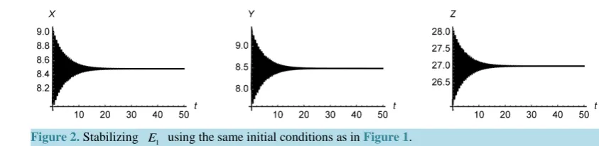
∆ = > . This occurs when k>0.694749. The system stabilizes faster as k increases. Figure

2 illustrates the stabilization using k=2.5.

With k=2.5, σ =10, =28, and b=8 3 system (3) has equilibrium points

1 2 3

8.48528 8.48528 27

6.70873 10.5072 26.4338 0.0794984 2.22069 0.0662031

X Y Z

E

E

E

− −

[image:5.595.90.512.79.182.2]

Figure 2. Stabilizing E₁ using the same initial conditions as in Figure 1.

The Jacobian of system (3) evaluated at each equilibrium point has the following eigenvalues

( )

( )

( )

1,2,3 1

2 3

15.72, 0.223353 10.17 16.1683, 0.000829684 8.8245

24.4271,10.9209, 2.66049

E i

E i

E

λ

− − ±

− ±

− −

J J J

Observe that the Jacobian confirms that E₁ is stable. Note that E₂ and E₃ are unstable.

This algorithm is well-suited to computer arithmetic and can be carried out at other equilibria. For example, rather than E₁, choose E₀=

(

0, 0, 0

)

and a control of the form −k X

(

−0

)

= −kX in the X-equation results in

270

k> as illustrated inFigure 3.

3.2. Y-Control

Generally, smaller k-values are considered “more efficient” than larger k-values. Thus, choosing E₀=

(

0, 0, 0

)

but a control of the form −k Y

(

−0

)

= −kY in the Y-equation results in k>27, which is more “efficient” than the linear control −kX in the X-equation used where we saw that k>270 was required. Incorporating the linear control into the Y-equation, we find that k>27 stabilizes the system as illustrated inFigure 4.

However, the method illustrated is trial-by-error, which makes it particularly well-suited for computer arithmetic. For example, choosing E₀=

(

0, 0, 0

)

and finding k-values for a control of the form −k Z

(

−0

)

= −kZ in the Z-equation is impossible. In this case, the characteristic polynomial of the Jacobian evaluated at E₀ is

( ) (

)

(

2

)

2.66667 1 1 270 11 1

p λ = + ⋅ + ⋅k λ − + ⋅ + ⋅λ λ , which has zeros λ = −₁ 22.8277 , λ =₂ 11.8277 , and

(

)

3 0.333333 8 3 k

λ = − − ⋅ : for every value of k, the Jacobian evaluated at E₀ has a positive eigenvalue so E₀ will be unstable.

4. The Rössler Attractor

The three-dimensional version of the Rössler attractor is

(

)

d d

d d

d d ,

X t Y Z

Y T X aY

Z t b Z X c

= − −

= +

= + −

(4)

where a, b, and c are positive constants.

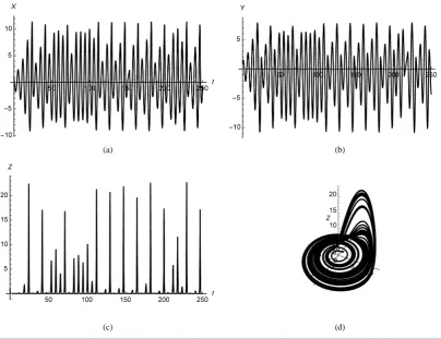
System (4) has been extensively studied and, consequently, its equilibria and the behavior of system (4) are well understood.Figure 5 illustrates chaos in the Rössler attractor using the parameter values a= =b 0.2 and

5.7

c= . Wang and Wu, [6], have applied a more complex controller than the one presented here to a four- dimensional hyperchaotic Rössler system.

For these parameter values, system (4) has the following equilibrium points

1 2

0.0070262 0.035131 0.035131 5.69297 28.4649 28.4649

X Y Z

E

E

[image:6.595.77.532.77.319.2] [image:6.595.110.515.332.643.2]

Figure 3. Stabilizing E0 with a control of the form −kX in the X-equation requires k>270. The initial conditions are x

( )

0 =0.1, y

( )

0 =0.1, and z

( )

0 =0.2.

Figure 4. Stabilizing E0 with a control of the form −kY in the Y-equation requires k>27. The initial condi- tions are the same as used in Figure 3.

(a) (b)

(c) (d)

Figure 5. Chaos in the Rössler attractor using “typical” parameter values and initial conditions,

( )

0

( )

0

( )

0 1.

X =Y =Z = (a) t vs. x; (b) t vs y; (c) t vs z; (d) x vs y vs z.

Following the same approach as in the previous example, we start by searching for a controller of the form

(

*

)

k X X

( )

1

1 1

1 0.2 0 .

0.035131 0 5.69297

k

E

− − −

 

 

=  

 ₋ 

 

J

To guarantee that the eigenvalues of J

( )

E₁ have negative real part, we apply the Routh-Hurwitz theorem.

In this case we must have that ∆ = ⋅ +₁ 1 k 5.49297>0, 2

2 5.49297k 31.2079k 6.25427 0

∆ = + − > , and

3 2

3 6.25427k 4.30038k 184.568k 35.5615 0

∆ = − − + − > . These equations are satisfied when

0.193796≤ ≤k 4.99383. Observe that if we look at a plot of the maximum part of the real part of the roots of the characteristic polynomial, p

( )

λ , of J

( )

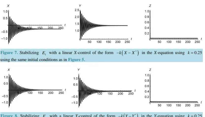
E₁ , we obtain the same interval as shown inFigure 6. Figure 7

illustrates stabilization using the k-value k=0.25.

For this example, choosing to stabilize E₁ using a control of the form −k Y

(

−Y*

)

in the Y-equation, where

*

0.035131

Y = − is the Y-component of E₁ is also successful. Using the same analysis, we find that ∆ >i 0

[image:7.595.199.423.295.430.2]

for i=1, 2, and 3 if k>0.194. Figure 8 illustrates stabilization using the k-value k=0.25.

Figure 6. A plot of the maximum value of the real part of the zeros of p

( )

λ as a function of k.

Figure 7. Stabilizing E1 with a linear X-control of the form

(

)

* k X X

[image:7.595.106.523.459.697.2]

− − in the X-equation using k=0.25 using the same initial conditions as inFigure 5.

Figure 8. Stabilizing E1 with a linear Y-control of the form

(

)

* k Y Y

It is not possible to stabilize the system using a control of the form −k Z

(

−Z*

)

in the Z-equation. The plot

of the maximum value of the real part of the roots of the characteristic polynomial, p

( )

λ , of J

( )

E₁ , in Figure 9 shows that the maximum value of the real part of any zero of p

( )

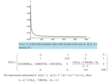
λ is always positive.

5. High-Himensional Rössler Attractors

Using the same notation as Musielak and Musielak, [1], the four dimensional Röseller system

d d

d d

d d

d d ,

X t Y Z

Y T X aY W Z t b XZ

W t cZ dW

= − −

= + +

= + = − +

(5)

where a, b, c, and d are positive constants can exhibit more complex behavior than system (4). System (5) is interesting because depending upon the parameter values and initial conditions chosen, the system can exhibit

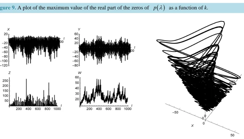
[image:8.595.200.440.318.459.2]

hyperchaos, which is illustrated inFigure 10 using the parameter values a=0.25, b=3, c=0.5, and d=0.05. On the other hand, adjusting the initial conditions can lead to dramatically different behavior as shown inFigure 11.

Figure 9. A plot of the maximum value of the real part of the zeros of p

( )

λ as a function of k.

Figure 10. The 4-dimensional Rössler system exhibiting hyperchaos. The initial conditions are X

( )

0 = −10,

( )

0 6

[image:8.595.115.514.456.684.2]

[image:9.595.107.528.80.257.2]

Figure 11. The behavior of the 4-dimensional system is highly dependent on the initial conditions. The initial conditions used are X

( )

0 =5, Y

( )

0 =0.5, Z

( )

0 = −0.5, and W

( )

0 = −0.5.

For these parameter values, system (5) has the following equilibrium points

1 2

5.40833 0.5547 0.5547 5.547 5.40833 0.5547 0.5547 5.547

X Y Z W

E b

E

− −

− −

The Jacobian of system (5) evaluated at each equilibrium point has the following eigenvalues

( )

( )

1,2,3,4

1

2

5.50404, 0.0510792 0.971052 , 0.103929 5.30896, 0.0493731 0.998687 , 0.101891

E i

E i

λ

±

− ±

J J

so both E₁ and E₂ are unstable. We illustrate stabilizing

(

* * * *

)

(

)

1 , , , 5.40833, 0.5547, 0.5547, 5.547

E = X Y Z W = − − . Keep in mind that we try to find the simplest linear

control that stabilizes the system. For this system, it is not possible to stabilize E₁ by incorporating a control of

the form −k X

(

−X*

)

into the X-equation because the Jacobian for the system dX dt= − − −Y Z k X

(

−X*

)

,

dY dt=X +aY+W , dZ dt= +b XZ , and dW dt= −cZ+dW evaluated at E₁ has characteristic polynomial

( )

2 2 3 3 4

0.540833 0.0676041 5.35952 1.635 2.0803 5.70833 5.70833 1 1

p

λ

= − k−

λ

+ k

λ

+

λ

− k

λ

−

λ

+ ⋅k

λ

+ ⋅

λ

and the plot of the maximum value of the real part of any root of p

( )

λ shown in Figure 12 shows us that there is

always a root with positive real part so E₁ will be unstable. Similarly, it is not possible to stabilize E₁ by

incorporating a control of the form −k Y

(

−Y*

)

into the Y-equation, a control of the form −k Z

(

−Z*

)

into

the Z-equation, or using a control of the form −k W

(

−W*

)

into the W-equation.

Next, we attempt using multiple controls. First, we try to find a control of the form −k₁

(

X −X*

)

in the

X-equation and a control of the form −k Y2

(

−Y*

)

in the Y-equation but find that there are no k1 and k2

values that will stabilize the system with this control.

Next, we try to find a control of the form −k₁

(

X −X*

)

in the X-equation and a control of the form

(

*

)

2

k Z Z

− − in the Z-equation,

(

*

)

1

dX dt= − − −Y Z k X −X , dY dT =X +aY+W,

(

*

)

2

[image:10.595.82.520.82.407.2]

Figure 12. A plot of the maximum value of the real part of the zeros of p

( )

λ as a function of k.

( )

1

1 2 1 1 2

2 1 1 2

1

1 1 0

1 0.25 0 1

.

0.5 2.70416 2

0.0128205 0.0693375 0.0512821 0 0

4

0 0 0.5 0.05

k

E k k k k

k k k k

k − − −         = _{− −} − + +  ₋     ₋    J

The characteristic polynomial of J

( )

E₁ is p

( )

λ

=

λ

4+b1

λ

3+b2

λ

2+b3

λ

+b4, where 2

1 1 1 2 1 2

2 2

2 1 2 1 1 2 1 2

2 2

3 1 2 1 1 2 1 2

4

0.5 7.00416 2 1.2

0.512821 3.0735 2.25256 3.3011 0.805128 4.05

0.153846 0.84455 1.13702 2.92117 2.08654 0.2

and 0.

b k k k k k

b k k k k k k k

b k k k k k k k

b

= + − − +

= − − + + −

= − + + − − +

=

We plot the region where the maximum value of the real part of any zero of p

( )

λ is negative inFigure 13

using the following algorithm.

(1) Given k₁ and k₂ find the zeros of p

( )

λ .

(2) Compute the real part of each zero and find the maximum real part of all zeros.

(3) Plot the region where the maximum value of the real part of any zero of p

( )

λ is less than or equal to

zero.

We find that we can control the system and stabilize E₁ using k₁=2 and k₂ =10. For these parameter values, the equilibrium points of the system are

1 2

5.40833 0.5547 0.5547 5.547 0.816654 12.6854 0.23547 2.3547

X Y Z W

E

E

− −

− − −

The Jacobian of this system evaluated at each equilibrium point has the following eigenvalues

( )

( )

1,2,3,4

1

2

10.8429, 1.35914, 0.345197, 0.0305914 4.77438, 1.18702, 0.165139 0.01376

E E i

λ

− − − − − − ± J J

[image:11.595.184.503.84.346.2]

Figure 13. In the shaded region, the real part of all the zeros of p

( )

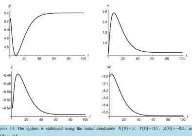
λ are less than or equal to zero.

Figure 14. The system is stabilized using the initial conditions X

( )

0 =5, Y

( )

0 =0.5, Z

( )

0 = −0.5, and

( )

0 0.5

W = − .

6. Conclusion

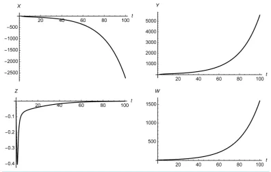
[image:11.595.117.513.366.645.2]

[image:12.595.114.511.84.335.2]

Figure 15. The control does not globally stabilize the system. The initial conditions are the same as those used inFigure 10.

as examples because they are very different models, but well studied and familiar to a wide audience. The simulations illustrated here show that the technique works on a wide range of dynamical systems, which we hope to further illustrate in later studies. Our simulations also indicate that it does not matter whether one uses the Routh-Hurwitz theorem or the characteristic polynomial to determined conditions on when all the eigenvalues of a matrix have negative real part. In future studies, we will focus on the physical interpretations of the controls that are introduced here as well as discuss conditions under which the control algorithm works or does not.

Computational Notes

The Mathematica, [7], notebooks that the authors used to carry out the calculations as well as generate the figures here are available from the authors by sending a request to Jim Braselton at

[email protected].

References

[1] Musielak, Z.E. and Musielak, D.E. (2009) High-Dimensional Chaos in Dissipative and Driven Dynamical Systems. International Journal of Bifurcation and Chaos, 19, 2823-2869.

[2] Chun, F.Y., Wang, H., Hu, Y. and Yin, J.W. (2012) Antisynchronization of a Novel Hyperchaotic System with Para-meter Mismatch and External Disturbances. Pramana-Journal of Physics, 79, 81-93.

[3] Li, Y. and Li, B. (2009) Chaos Control and Projective Synchronization of a Chaotic Chen-Lee System. Chinese Jour-nal of Physics, 47, 261-279.

[4] Tan, X., Zhang, J. and Yang, Y. (2003) Synchronizing Chaotic Systems Using Backstepping Design. Chaos, Solitons, Fractals, 16, 37-45.

[5] Vieira, D. and Lichtenberg, A.J. (1966) Controlling Chaos Using Nonlinear Feedback with Delay. Physical Review E,

54, 1200-1207.

[6] Wang, X.Y. and Wu, X.J. (2006) Tracking Control and Synchronization of Four-Dimensional Hyperchaotic Rössler System. Chaos, 16, 03312. http://dx.doi.org/10.1063/1.2213677