DOI: 10.1140/epjb/e2003-00294-0
T
HE
E
UROPEAN
P
HYSICAL
J
OURNAL
B
Short-distance wavefunction statistics in one-dimensional
Anderson localization
H. Schomerusa and M. Titov
Max-Planck-Institut f¨ur Physik komplexer Systeme, N¨othnitzer Str. 38, 01187 Dresden, Germany Received 10 July 2003
Published online 15 October 2003 – cEDP Sciences, Societ`a Italiana di Fisica, Springer-Verlag 2003 Abstract. We investigate the short-distance statistics of the local density of statesνin long one-dimensional disordered systems, which display Anderson localization. It is shown that the probability distribution functionP(ν) can be recovered from the long-distance wavefunction statistics, if one also uses parameters that are irrelevant from the perspective of two-parameter scaling theory.
PACS. 72.15.Rn Localization effects (Anderson or weak localization) – 05.40.-a Fluctuation phenomena, random processes, noise, and Brownian motion – 42.25.Dd Wave propagation in random media – 73.20.Fz Weak or Anderson localization
1 Introduction
Wave localization in a disordered potential is the most striking hallmark of systematic interference by multiple coherent scattering [1–8]. Systematic constructive inter-ference in a spatially localized region results in a con-finement of the wavefunction, which decays exponentially away from the localization center (with a decay lengthlloc, the localization length), in contrast to the extended waves in constant or spatially periodic potentials. Localization comes along with large fluctuations of the wavefunction, which can be induced by changing the disorder config-uration. The wavefunction statistics can be probed, e.g., globally across a system of finite lengthLsysby the dimen-sionless conductance (transmission probability)g, and in-side a semi-infinite system (Lsys=∞) by the local density of states ν at a distanceLopen to the opening.
Theories of localization often focus on the long-distance wavefunction statistics, where a high degree of universality prevails. For instance, distribution functions are restricted to log-normal forms as a consequence of the central-limit theorem, which leads to two-parameter scaling (TPS) [9]. Consequentially, for the local density of states, the probability distribution function P(ν) is characterized by the mean logarithmC1(ν) ≡ −lnνand its variance C2(ν) ≡ var lnν. The TPS observation has found many applications [10–16]. An even enhanced de-gree of universality arises in the random-phase approxi-mation (RPA), where single-parameter scaling (SPS) ap-plies [17–20], and both parameters further are connected,
a e-mail:[email protected]
e.g.byC2(ν)∼2C1(ν)for one-dimensional systems [21–23]. (It was recognized very early that SPS breaks down for strong disorder, see,e.g., Ref. [24].)
In this paper we point out a connection of the long-distance statistics to the short-long-distance statistics in the one-dimensional Anderson model of localization, probed by the local density of states ν. Namely, we find that the distribution functionP(ν) for short distances reliably can be approximated with the help of parameters that are ex-tracted from the long-distance limit, including parameters (besidesC1(ν) andC2(ν)) that are irrelevant, from the per-spective TPS, for the long-distance wavefunction statistics themselves.
We start this paper by an analysis ofP(ν) andP(g) within the concepts of large-deviation statistics [25], which goes beyond the central-limit theorem, and identify quan-tities Cn, n ≥ 3, which are irrelevant for the long-distance wavefunction statistics, but will turn out to be useful for the short-distance wavefunction statistics. Each quantity defines its own length scale by its asymptotic slope cn = limL→∞dCn/dL (where L ≡ Lsys for g and
L ≡ Lopen for ν), in analogy to the relation between
C1 ∼2L/lloc and the localization lengthlloc. The length scales obtained fromνandgcoincide. The constant offsets
dn= limL→∞Cn−Lcn are shown to contain information
on the reflection phase, which allows to test the RPA. Then we discuss thatP(ν) for short distancesLopen lloc can be reconstructed from the parameterscn anddn.
observations for the short-distance statistics lead us to conclude that the cumulantsCn are useful characteristics
of localized wavefunctions, even though they are not rele-vant in the long-distance limit because of TPS.
Finally, we analytically and numerically investigate the parameters cn and dn in various regimes of the
one-dimensional Anderson model.
The paper is organized as follows: In Section 2 we de-scribe the general implications of large-deviation statis-tics for the scaling of the distribution functionsP(g) and
P(ν), and identify the parameters cn and dn in the
cu-mulantsCn,n≥3. In Section 3 we specialize to the
one-dimensional Anderson model. In order to motivate subse-quent considerations, we first illustrate in Section 3.1 the length dependence of the cumulantsCnby numerical
sim-ulations. Then (Sect. 3.2) we briefly review the analytical theory for the asymptotic slopes cn [26, 27] and extent it
to the case of competition between onsite disorder and offsite disorder close to the band center. We also present the theory for the asymptotic offsetsdn. In Section 3.3 we
investigate the dependence of the parameters in various regimes of the Anderson model. Our conclusions are given in Section 4.
In order to facilitate a parallel discussion of the statis-tics of g and ν, we use the common notation L ≡ Lsys when considering g and L ≡ Lopen when consid-ering ν. One has to bear in mind that in the latter case, Lsys =∞and hence one always discusses localized wavefunctions, while in the former case this is true only forL≡Lsyslloc.
2 Large-deviation statistics
Large-deviation statistics often is introduced as the third and final step in a progressively refined analysis of the asymptotic behavior of probability distribution functions, where the first step is the law of large numbers and the second is the central-limit theorem. In localization, the law of large numbers certifies that the Lyapunov exponent
γ = C1(g)/2L is self-averaging in the limit L → ∞ [28], with asymptotic value limL→∞γ=lloc−1. The central-limit
theorem delivers a statement about the finite-length cor-rections to this asymptotic value, which are characterized by C2(g): The variance varγ =C2(g)/L2 decreases asymp-totically as L−1. Presently, we find it useful not address the Lyapunov exponents, since these are defined with help of the system lengthL, but to rely on quantities that only involve g or ν, like C1(g), C2(g), C1(ν), and C2(ν). The law of large numbers and the central-limit theorem predict a linear growth of these quantities with L. The full pic-ture is unfolded in the framework of large-deviation statis-tics [25]: All cumulants can increase linearly with length or distance,
Cn(g)=(−lng)n ∼cn(g)L+d(ng) (Llloc), (1a)
Cn(ν)=(−lnν)n ∼cn(ν)L+d(nν) (Llloc), (1b)
where the coefficients dn are the subleading corrections
that can be neglected in the asymptotic limit, but will be
seen to encode information on the reflection phase that allows to test the validity of the RPA. For the conduc-tance g, the linear scaling of the cumulants Cn(g) with L
and the connection of thed(ng)to reflection phases also has
been found in a constructive theory by Roberts [29]. The parameterscn can be extracted from the averages
c(g)(ξ) =− lim
L→∞
1
Llng
−ξ= n
ξn n!c
(g)
n (2)
(or equivalently for ν) as function of the continuous parameter ξ. Note the exponential dependence of the moments on L due to localization, in contrast to the power-law dependence in the critical regime around a metal-insulator transition [7].
This paper is centered around our numerical observa-tion in Secobserva-tion 3 that equaobserva-tion (1b) holds even for short distances to the opening Lopen lloc, and hence can be used in regions where the central-limit theorem does not apply. This makes the parameters cn anddn with n≥3
observable in the distribution functionP(ν), while in the long-distance behavior onlyc1andc2are relevant param-eters [9].
Presently, analytical results for the distribution func-tionP(g) and P(ν) for short distances are only available in the regime of single-parameter scaling. The local den-sity of states obeys a strict log-normal distribution for all distances [23, 30], and hence complies with our central ob-servation. Equation (1a) cannot be extended to short dis-tances, even in the regime of single-parameter scaling [21]; for studies outside this regime see,e.g., references [13, 26].
3 One-dimensional Anderson model
The previous Section 2 put forward some very general ar-guments from large-deviation statistics. The relevance of the asymptotically defined parameterscn (anddn),n≥3
for finite-distance wavefunction statistics, and the ques-tion whether these parameters indeed contain informaques-tion that is independent from what is encoded in the parame-tersc1andc2, only can be answered by a direct investiga-tion. In the following we analyze the wavefunction statis-tics in the one-dimensional Anderson model [3], given by the Schr¨odinger equation discretized on a chain (lattice constanta≡1)
tl−1ψl−1+tlψl+1= (Vl−E)ψl, (3)
where the hopping matrix elements tl and the disorder potential Vl are random. We assume box distributions
with tl = t, Vl = 0, tltm = t2 + 12Dtδlm, and VlVm = 2DVδlm. Without any restriction we can set t= 1, which fixes the energy scale in the dispersion rela-tionE(k) =−2 coskof the clean system (Dt=DV = 0). The disorder strength will be characterized by the pertur-bative mean-free path [31]
and the balance between onsite and offsite disorder will be characterized by the parameter
δ= (DV −Dt)/(DV +Dt). (5)
First we present the results of numerical simulations to illustrate the usefulness of the cumulantsCn. Next, in
or-der to give a flavor for the mechanism behind the asymp-totic linear growth (1) of the cumulants for the specific case of wavefunction localization, we extent the analyti-cal theory of references [26, 27] for the asymptotic slopes
cn to the case of competition of onsite- and offsite
disor-der close to the band centerE = 0, and also present the theory for the offsets dn. The extension equips us with a means to violate SPS, which is finally compared to other means in order to determine the mutual (in)dependence of the parameterscn anddn.
3.1 Numerical illustration of the cumulants Cn
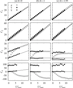
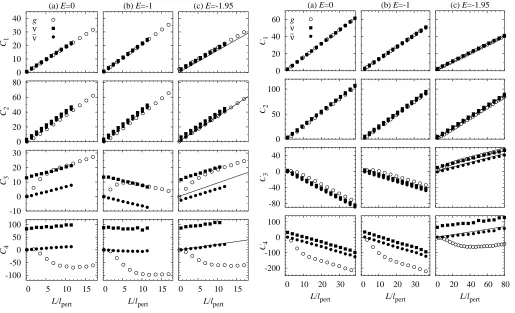
Here we illustrate the length dependence of the cumu-lants Cn by the results of numerical computations in en-sembles of 106−108 disorder realizations. The results for different strengths of onsite disorder (δ= 1) are presented in Figure 1 (lpert = 300), Figure 2 (lpert = 24), and Fig-ure 3 (lpert= 1.5). Three representative values of energy are chosen: (a) E = 0 at the band center, (b) E = −1 in the SPS region, (c)E=−1.95 close to the band edge. [The constant perturbative mean free pathlpertin any fig-ure has been obtained by adjusting the disorder strength according to equation (4); for values see the figure cap-tions.] The significance of these three regions of energy will be discussed in the following Section 3.2. Plotted as a function of length are the cumulants Cn calculated
from g andν, as well as from the ‘mesoscopic’ local den-sity of states ˜ν, which is obtained from ν by averaging over a Fermi wavelength λF = 2π/arccos(−E/2) (with
λF = 4 forE = 0, λF= 6 for E =−1, and λF ≈28 for E=−1.95). The mesoscopic density of states accounts for a limited resolution that may be encountered in an exper-iment. It discards the nodes of the wavefunction (whose impact strongly depends on the dimensionality of the sys-tem) and only captures the smoothly varying envelope (which is more robust).
The cumulants all increase linearly for L lloc, and one may associate a length scale limL→∞2L/Cn = 2/cn
to each of them. The slopes cn are identical for all three underlying objects, and hence the sets of parameters
{c(ng)}={cn(ν)}={c(˜nν)} ≡ {cn} coincide.
As advertised above, the cumulants Cn(ν) and Cn(˜ν)
increase linearly already for small L lloc (moreover, the offsets for ˜ν are vanishingly small), while the cumu-lantsCn(g)become linear only after some transient length, see reference [13] (these cumulants also have a finite off-set d(ng)). This means that the asymptotically defined pa-rametersc(nν)and d(nν)can be used to estimate the short-distance behavior of Cn(ν) and Cn(˜ν). In order to estimate the distribution functions, parameters withn≥3 have to
0 10 20 30
C1
(a) E=0
g ν ~ ν
0 20 40 60
C2
0 10 20 30
C3
-100 -50 0 50 100
0 5 10
C4
L/lpert
(b) E=-1
0 5 10
L/lpert
(c) E=-1.95
0 5 10
[image:3.595.302.554.94.397.2]L/lpert
Fig. 1. CumulantsCncalculated fromgas a function ofL≡
Lsys, and fromν, ˜νas a function ofL≡Lopen. The data points are obtained by a numerical simulation of the one-dimensional Anderson model with onsite disorder, forE = 0,DV = 1/75, (left panels), E = −1 , DV = 1/100 (middle panels), and
E =−1.95,DV = 0.0006583 (right panels). This corresponds to weak disorder, with a perturbative mean-free path oflpert= 300 in all cases (see Eq. (4)). The lines are analytical weak-disorder predictions of the asymptotic linear behavior Cn ∼
cnL, taken from reference [26] for E = 0 and following the RPA forE=−1 andE=−1.95.
be included, since the central-limit theorem does not yet apply for short distances. This is displayed in Figure 4, which comparesP(lnν) forL=lloc/2,E=−1,lpert= 24 with a normal distribution, which only accounts for C1(ν)
andC2(ν), and with a generalized normal distribution (the so-called Pearson system [32]),
P(x) =C(a+bx+cx2)−1/2c
×exp
(b+ 2cm) arctan[(b+ 2cx)/√4ac−b2]
c√4ac−b2
, (6)
0 10 20 30 40
C1
(a) E=0
g ν ~ ν
0 20 40 60 80
C2
-10 0 10 20 30
C3
-100 -50 0 50 100
0 5 10 15
C4
L/lpert
(b) E=-1
0 5 10 15
L/lpert
(c) E=-1.95
0 5 10 15
[image:4.595.43.558.96.409.2]L/lpert
Fig. 2. Same as Figure 1, but for stronger disorder with
lpert= 24:DV = 1/6 (left),DV = 1/8 (middle),DV = 0.00823 (right). The lines in the right panels (c) are the analytic pre-dictions for the given disorder strength close to the band edge, taken from reference [27].
3.2 Analytical theory for the slopes cn and offsets dn
3.2.1 Slopes cn
Recently [26, 27], we have been able to extent Halperin’s phase formalism [22, 33], which allows to calculatellocand hencec1, to all slopescn. This formalism can be applied
for arbitraryλF/lpert,i.e., also for relatively strong disor-der, as long aslpert1 (the lattice constant, set to unity in this paper). Other formalisms like the supersymmet-ricσmodel and the Berezinskiˇı technique are rather more restrictive and cannot directly address the logarithm ofg
andν. It turned out that three different regions of energy have to be distinguished in the one-dimensional Ander-son model. For energies 2− |E|D2/3 close to the band edge, corresponding to relatively strong disorder, the RPA fails and the distribution function deviates from the strict log-normal form [27]. RPA fails also for energies|E|D
close to the band-center [34], and the distribution func-tion again deviates from the strict log-normal form [26], in generalization of the Kappus-Wegner anomaly ofllocat
E = 0 [24, 35, 36]. For other energies inside the band, the RPA is justified, and SPS holds, for weak disorder.
0 20 40 60
C1
(a) E=0
g ν ~ ν
0 50 100
C2
-80 -40 0 40
C3
-200 -100 0 100
0 10 20 30
C4
L/lpert
(b) E=-1
0 10 20 30
L/lpert
(c) E=-1.95
0 20 40 60 80
L/lpert
Fig. 3. Same as Figures 1 and 2, but for stronger disorder with lpert = 1.5: DV = 8/3 (left), DV = 2 (middle), DV = 0.1316 (right). The lines in the right panels (c) are the analytic predictions for the given disorder strength close to the band edge, taken from reference [27].
0 0.05 0.1 0.15 0.2 0.25
-10 -8 -6 -4 -2 0 2 4 6
P(ln
ν
)
ln ν
data Pearson normal
Fig. 4. The probability distribution function P(lnν) from a numerical simulation (data points) in the Anderson model with
[image:4.595.311.553.493.672.2]Offsite disorder adds another means to depart from SPS at the band center, since the balance parameter δ
interpolates between the Kappus-Wegner anomaly atδ= 1 (Dt= 0) and the Dyson singularity atδ=−1 (DV = 0), which results in total delocalization [37–41]. In the vicinity of the band center, we derive the following Fokker-Planck equation for the joint distribution function P(u, α;L) of
u −lng −lnν, and the phase αfor reflection from the system:
(DV +Dt)−1∂P ∂L =
∂α
δ
2s2α−ε
+∂α2(1 +δc2α)
−1
2∂u(1 +δc2α) + 1 2∂
2
u(1−δc2α) +∂u∂αδs2α
P,
(7)
wheresx= sinx,cx= cosx,ε=E/(DV+Dt), and∂ de-notes partial derivatives. Forδ= 1, this equation has been used to study the wavefunction statistics at the Kappus-Wegner anomaly [27]. Forδ=−1,E= 0, one recovers the delocalization at the Dyson anomaly. At the balance point of onsite and offsite disorder δ = 0, the variables uand
α decouple. For L → ∞ the reflection phase α becomes completely random, while P(u) precisely takes the form of SPS, with asymptotic slopes c2 = 2c1 and cn = 0 for n ≥ 3. Hence, somewhat surprisingly, we find that RPA and SPS hold true by a particularly simple mechanism just in between the two abovementioned anomalies.
Away from the novel SPS pointδ= 0, but for disor-der still small, the asymptotic behavior of the distribution function can be analyzed by introducing into equation (7) the large-deviation ansatz
P(u, α;L) =
+i∞
−i∞ dξ
2πi ∞
k=0
exp[c(ξ)L−ξu]f(α;ξ). (8)
Here c(ξ) = nξncn/n! is the generating function of
the slopes of the cumulants, see equations (1) and (2), and f(α;ξ) has to be periodic and normalizable with re-spect toα. We arrive at a differential equation
c(ξ)f(α;ξ)
DV +Dt =
∂α
δ
2s2α−ε
+∂α2(1 +δc2α)
+ξ
2(1 +δc2α−2∂αδs2α) +
ξ2
2 (1−δc2α)
f(α;ξ),
(9)
in which the slope-generating functionc(ξ) appears as an eigenvalue, whilef(α;ξ) appears as an eigenfunction. The slopes cn now can be calculated iteratively by
expand-ing c(ξ) andf(α;ξ) order by order inξ, following refer-ences [26, 27]. Away from the SPS point δ = 0 but for
|E| DV +Dt, the slopes cn take finite values, in
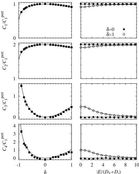
com-pliance with equation (1). Our analytical results are con-firmed by numerical computations in Figure 5.
3.2.2 Constant offsets dn
The offsets d(nν) ≈Cn(ν)(L = 0) can be calculated by ex-pressing the local density of statesν(L) in terms of the
0 1
C1
/C
1
pert
1 2
C2
/C
1
pert
0 1
C3
/C
1
pert
0 1 2 3 4
-1 0 1
C4
/C
1
pert
δ
δ=0 δ=1
0 2 4 6 8 10
[image:5.595.313.541.94.379.2]|E|/(DV+Dt)
Fig. 5. Cumulants Cn (in units of C1pert = 2L/lpert) in the asymptotic limitLlloc, as a function of the balance param-eter δ for energy E = 0 (left panels), and as a function ofE for δ= 0 andδ= 1 (right panels). Results of numerical simu-lations withlpert= 300 are compared to the predictions of the analytical theory.
flection coefficientsrR(rL) from the segment of the wire to the right (left) of the pointLat whichνis calculated [30],
ν(L) = Re(1 +rL)(1 +rR)
1−rLrR , (10)
where we normalizedν(L)= 1 (which amounts to mul-tiplication by a constant factorπ√4−E2). ForL= 0 and the opening of the wire oriented to the left,rL= 0 because there is no reflection from the opening, andrR= exp(iα), where α is the phase of reflection from the semi-infinite system. Hence, the numbers
d(nν)≈Cn(ν)(L= 0) =[−ln(1 + cosα)]n (11)
characterize the distribution of the reflection phase αof the semi-infinite system [30], and allow to assess the va-lidity of the RPA, which predictsd(1ν)= ln 2,d2(ν)=π2/3,
d(3ν) = 12ζ(3) (with the Riemann ζ function), d(4ν) = 14π4/15.
The offsets d(˜nν) ≈Cn(˜ν)(L = 0) vanish independently of the RPA since in terms of the reflection matrices intro-duced above
˜
ν(L) = Re1 +rLrR
1−rLrR, (12)
-3 -2 -1 0 1 2 3
X3
(
∞
)
(a) δ varies, E=0, lpert=300
δ<0 δ>0 analytics
(b) δ=1, E varies, lpert>>1
|E| ≈ 0 |E| ≈ 2
(c) δ=1, E fixed, lpert=1.5 - 300
E=0 E=-1 E=-1.95 fit
(d) combined results
-6 -4 -2 0 2 4
1.6 1.8 2.0 2.2 2.4
X4
(
∞
)
X2(∞)
1.6 1.8 2.0 2.2 2.4
X2(∞)
1.6 1.8 2.0 2.2 2.4
X2(∞)
1.6 1.8 2.0 2.2 2.4
[image:6.595.45.550.94.310.2]X2(∞)
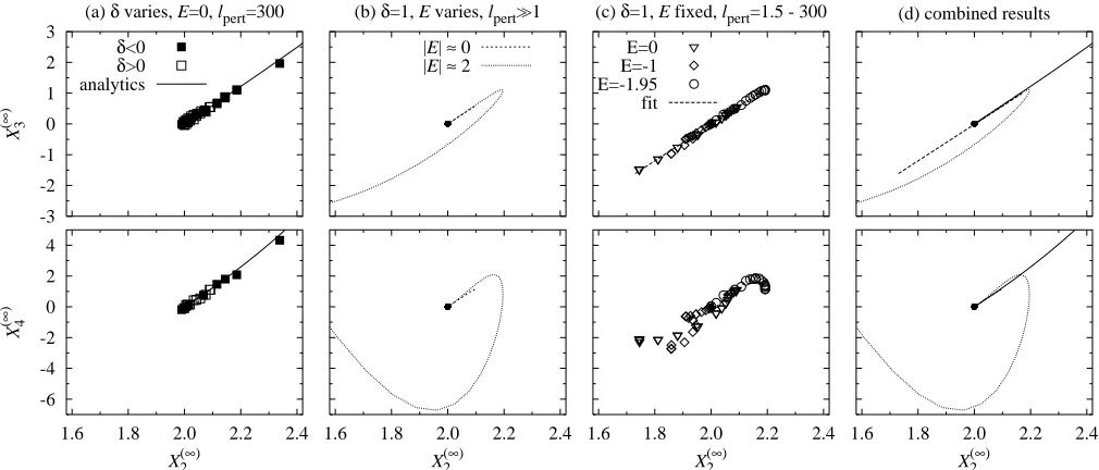
Fig. 6. Dependence of the parameters X3(∞) and X4(∞) on X2(∞) for various ways to depart from SPS (SPS conditions are indicated by the dot at coordinates (2,0)). (a) The balance of weak onsite and offsite disorder is changed at the center of the band, E = 0. The curve is the prediction of the analytical theory, while data points are obtained by numerical simulations. (b) Analytical results as energy is varied at a fixed strength of onsite disorder, withlpert1 butlpert/λFarbitrary, around the band center (E= 0) and around the band edge (|E| ≈2). (c) Numerics and linear fits for variable strength of onsite disorder at three different values of the energy. (d) Comparison of the curves in (a-c).
The offsetsd(ng) are obtained by considering the com-position law tR+L = tR(1 − rLrR)−1tL for the series transmission through two long segments R and L. The reflection coefficients now are equivalent phase factors
rR,L = exp(iαR,L). We equate the cumulants of both sides
and insert the asymptotics (1). The constant offsets follow asd(ng)= (−1)n{ln[2−2 cos(αR+αL)]}n. In the RPA,
d(1g) = 0 and dn(g) = (−1)nd(nν). This is clearly displayed in Figure 1. Beyond the RPA, the d(ng) and d(nν) contain equivalent information on the reflection-phase distribution functionP(α), but no longer are simply related.
3.3 Independence of the parameters
Now we turn to the question of the mutual independence of the parameterscn, as we violate the conditions for SPS.
A convenient set of parameters beyond the SPS quan-tityC1is formed by the ratiosXn =Cn/C1, which
asymp-totically acquire the constant values
lim
L→∞Xn=X (∞)
n =cn/c1. (13)
In RPA and SPS, only one effective parameter C1 sur-vives sincec(2g)=c2(ν)= 2c1(g)= 2c(1ν),i.e.,X2(∞)= 2, and moreoverc(ng)=c(nν)= 0 forn≥3, which gives a picture
consistent with SPS. However, beyond this approximation the cumulantsCn withn≥3 generally may increase
lin-early with L, and hence can be of the same order as C1
andC2, such that allXn(∞)are of order unity. Notice that the asymptotic valueXn(∞) is well approximated byXn(˜ν)
even for L lloc, since the cumulantsCn(˜ν) are linear al-ready for smallL and the offsetsd(˜nν)vanish.
In Figure 6 we plot the asymptotic ratios of cumulants
X3(∞)andX4(∞)as function ofX2(∞), while we vary:
(a) the balance parameter δ at E = 0 (a i) from 0 to 1 and (a ii) from 0 to−1;
(b) energy for fixed onsite disorder (b i) around E = 0 and (b ii) around|E|= 2; and
(c) the disorder strength from lpert = 300 to lpert = 1.5 at δ = 1 for the three values of energy (c i) E = 0, (c ii)E=−1, and (c iii)E=−1.95.
In the cases (a) and (b) we show the results of the an-alytical procedure described above, while for (c) we show the result of the numerical simulations. For illustration of the predictive power of the theory presented in the pre-vious Section 3.2, numerical results are also displayed for case (a).
Of particular interest is the curve for case (b ii), for en-ergies close to the band edge, which also applies to strong disorder,D2/32− |E|[27]. (See also the data points for case (c iii).) In this case the curves Xn(∞)(X2(∞)) depart from the seemingly unique functional behavior obtained in the other cases. Hence, we are led to conclude that at least for sufficiently strong disorder X3(∞) and X4(∞) are not uniquely determined by X2(∞). Since the SPS quan-tity C1 is always an independent scaling parameter, alto-gether more than two quantities are needed to characterize the distribution functionP(ν) for short distancesLlloc
4 Conclusions
We observed that theshort-distancestatistics of localized wavefunctions inside a long one-dimensional disordered system can be recovered from the long-distance statis-tics, but in general are characterized by more than the two parameters (a meanC1 and a varianceC2) that suf-fice to describe the long-distance statistics themselves. These additional parameters have been obtained from the higher cumulants Cn of lnν, where ν is the local
den-sity in a semi-infinite system. The additional parameters in the Cn can be neglected when considering the case of weak disorder and generic energies within the band: Then
C1∼C2/2∝L, and alsoCn=O(L0) forn≥3 take
uni-versal values, which results in a picture consistent with single-parameter scaling even in the short-distance wave-function statistics.
With three-dimensional systems in mind, it would be desirable to investigate the relation of the parameters from large deviation statistics to the scaling parameters at the metal-insulator transition, which may be established by multi-fractal analysis when this transition is approached from the localized regime.
Another potential application of the higher cumulants is to use them for detecting spatial correlations in the disorder, since the higher cumulants are sensitive to more-point wavefunction correlations. This offers a natural ex-tension of a previous investigation [42], which demon-strated that deviations from randomness due to spatial three-point correlations (such as displayed by a folded Fibonacci sequence) cannot be detected by the conven-tional wavefunction statistics.
References
1. P. Sheng, Scattering and Localization of Classical Waves in Random Media(World Scientific, Singapore, 1990) 2. R. Berkovits, S. Feng, Phys. Rep.238, 135 (1994) 3. P.W. Anderson, Phys. Rev.109, 1492 (1958)
4. P.A. Lee, T.V. Ramakrishnan, Rev. Mod. Phys. 57, 287 (1985)
5. B. Kramer, A. MacKinnon, Rep. Prog. Phys. 56, 1469 (1993)
6. C.W.J. Beenakker, Rev. Mod. Phys.69, 731 (1997) 7. M. Janssen, Phys. Rep.295, 1 (1998)
8. A.D. Mirlin, Phys. Rep.326, 259 (2000)
9. A. Cohen, Y. Roth, B. Shapiro, Phys. Rev. B38, 12125 (1988)
10. P. Markoˇs, B. Kramer, Phil. Mag. B68, 357 (1993); Ann. Physik (Leipzig)2, 339 (1993)
11. L.I. Deych, D. Zaslavsky, A.A. Lisyansky, Phys. Rev. Lett. 81, 5390 (1998)
12. L.I. Deych, A.A. Lisyansky, B.L. Altshuler, Phys. Rev. Lett.84, 2678 (2000); Phys. Rev. B64, 224202 (2001)
13. L.I. Deych, M.V. Erementchouk, A.A. Lisyansky, Phys. Rev. Lett. 90, 126601 (2003); Phys. Rev. B 67, 024205 (2003)
14. P.-G. Luan, Z. Ye, Phys. Rev. E64, 066609 (2001) 15. J.W. Kantelhardt, A. Bunde, Phys. Rev. B 66, 035118
(2002)
16. S.L.A. de Queiroz, Phys. Rev. B66, 195113 (2002) 17. E. Abrahams, P.W. Anderson, D.C. Licciardello, T.V.
Ramakrishnan, Phys. Rev. Lett.42, 673 (1979)
18. P.W. Anderson, D.J. Thouless, E. Abrahams, D.S. Fisher, Phys. Rev. B22, 3519 (1980)
19. B.L. Altshuler, V.E. Kravtsov, I.V. Lerner, Pis’ma Zh. Eksp. Teor. Fiz. 43, 342 (1986) [JETP Lett. 43, 441 (1986)]; Zh. Eksp. Teor. Fiz. 91, 2276 (1986) [Sov. Phys. JETP64, 1352 (1986)]
20. K. Slevin, P. Markos, T. Ohtsuki, Phys. Rev. Lett. 86, 3594 (2001); Phys. Rev. B67, 155106 (2003)
21. A.A. Abrikosov, Solid State Commun.37, 997 (1981) 22. I.M. Lifshitz, S.A. Gredeskul, L.A. Pastur,Introduction to
the Theory of Disordered Systems(Wiley, New York, 1988) 23. B.L. Altshuler, V.N. Prigodin, Zh. Eksp. Teor. Fiz.95, 348
(1989) [Sov. Phys. JETP 68, 198 (1989)] 24. M. Kappus, F. Wegner, Z. Phys. B45, 15 (1981)
25. R.S. Ellis, Entropy, Large Deviations and Statistical Mechanics (Springer, New York, 1985)
26. H. Schomerus, M. Titov, Phys. Rev. B 67, 100201(R) (2003)
27. H. Schomerus, M. Titov, Phys. Rev. E 66, 066207 (2002) 28. V.I. Oseledec, Trudy Moskov. Mat. Obshch.19, 179 (1968)
[T. Moscow Math. Soc.19, 197 (1968)]
29. P.J. Roberts, J. Phys.: Condens. Matter4, 7795 (1992) 30. H. Schomerus, M. Titov, P.W. Brouwer, C.W.J.
Beenakker, Phys. Rev. B65, 121101(R) (2002)
31. D.J. Thouless, in Ill-Condensed Matter, edited by R. Balian, R. Maynard, G. Toulouse (North-Holland, Amsterdam, 1979)
32. K. Pearson, Phil. Trans. A216, 429, (1916); C.C. Craig, Ann. Math. Stat.7, 16 (1936); C. Craig, in Mathematics of Statistics Pt. 2, edited by J.F. Kenney, E.S. Keeping (Van Nostrand, Princeton, NJ, 1951), p. 107
33. B.I. Halperin, Phys. Rev. B139A, 104 (1965)
34. A.D. Stone, D.C. Allan, J.D. Joannopoulos, Phys. Rev. B 27, 836 (1983)
35. B. Derrida, E. Gardner, J. Phys. France45, 1283 (1984) 36. I. Goldhirsch, S.H. Noskowicz, Z. Schuss, Phys. Rev. B49,
14504 (1994)
37. G. Theodorou, M.H. Cohen, Phys. Rev. B13, 4597 (1976) 38. T.P. Eggarter, R. Riedinger, Phys. Rev. B18, 569 (1978) 39. A.A. Gogolin, V.I. Melnikov, Zh. Eksp. Teor. Fiz.73, 706
(1977) [Sov. Phys. JETP 46, 369 (1977)]
40. A.A. Gogolin, Zh. Eksp. Teor. Fiz. 77, 1649 (1979) [Sov. Phys. JETP50, 827 (1979)]
41. A. Bovier, J. Stat. Phys.56, 645 (1989)