Munich Personal RePEc Archive
On the Spectral Properties of Matrices
Associated with Trend Filters
Luati, Alessandra and Proietti, Tommaso
Department of Statistics, University of Bologna, SEFEMEQ,
University of Rome "Tor Vergata"
10 November 2008
Online at
https://mpra.ub.uni-muenchen.de/11502/
On the Spectral Properties of Matrices Associated with
Trend Filters
Alessandra Luati Department of Statistics
University of Bologna
Tommaso Proietti S.E.F. e ME. Q.
University of Rome “Tor Vergata”
Abstract
This note is concerned with the spectral properties of matrices associated with linear smoothers. We derive analytical results on the eigenvalues and eigenvectors of smoothing ma-trices by interpreting the latter as perturbations of mama-trices belonging to algebras with known spectral properties, such as the Circulant and the generalised Tau. These results are used to characterise the properties of a smoother in terms of an approximate eigen-decomposition of the associated smoothing matrix.
Keywords Signal extraction; Smoothing; Boundary conditions; Matrix algebras.
JEL codes:C22.
1
Introduction and motivations
This note is concerned with linear smoothers that provide the estimator of a signal,yˆ, as linear combinations of the observations:
ˆ
y=Sy. (1)
HereSis then×nsmoothing matrix associated with the filter andyis ann×1vector of observed values.
The rows ofS define the equivalent kernel of the smoother and arise from a number of both parametric and nonparametric approaches: (i) local polynomial regression (see Fan and Gjbels, 1996); (ii) filtering with low-pass filters designed in the frequency domain (see for instance Bax-ter and King, 1999, and Christiano and Fitzgerald, 2003); (iii) wavelet multiresolution analysis (Percival and Walden, 2000); (iv) penalized least squares (Green and Silverman, 1994); (v) linear mixed models using parametric representations for the signal (Whittle, 1983).
The eigen-decomposition ofSprovides a useful characterisation of the properties of a smoother; see Buja, Hastie and Tibshirani (1989), Hastie and Tibshirani (1990) and Ruppert, Wand and Car-roll, (2003). In the symmetric case, if S = Pn
i=1λiviv′i is the spectral decomposition of the smoothing matrix, whereλi are the ordered eigenvalues andvi the corresponding eigenvectors, we can meaningfully decompose the fit asyˆ =Pn
what sequences are preserved or compressed via a scalar multiplication and αi are the specific coefficients of the projection ofyonto the space spanned by the eigenvectorsvi,y=Pn
i=1αivi. Moreover, tr(S) = Pn
i=1λiprovides the number of degrees of freedom of a smoother, which is a measure of the equivalent number of parameters used to obtain the fityˆthat allows to compare alternative filters according to their degree of smoothing. A related notion is that of the rank of a smoother.
The eigen-decomposition of a smoothing matrix is most informative if the matrix S is sym-metric. In fact, when this is not the case, the eigenvalues and eigenvectors are complex and the interpretation of the spectral decomposition is not direct. In the nonsymmetric case Buja, Hastie and Tibshirani (1989) propose to analyse of the singular value decomposition ofS, since the sin-gular values are always real as they represent the squared root of the eigenvalues of the symmetric
SS′. Nevertheless, the right eigenvectors differ from the left eigenvectors and it is no longer clear
what components are passed through by the filter or compressed.
Symmetric smoothers arise in the context of spline smoothing and from optimal signal extrac-tion for certain classes of parametric linear mixed models (see e.g. Whittle, 1983). A relevant case in macroeconomics is the Leser-Hodrick-Prescott filter (see Leser, 1951, Hodrick and Prescott, 1997). However, nonsymmetric smoothing matrices arise in a variety of important contexts as in local polynomial regression, and more generally, when a finite impulse response (FIR) filter is designed according to some constructive principle. A common characteristic of the approaches leading to FIR filters is that a constructive principle (e.g. band–pass filtering, Baxter and King, 1999, Percival and Walden, 2000, or local polynomial reproduction, Fan and Gjibels, 1996, Cleve-land and Loader, 1996) yields a two–sided filter for the central observations, using a specified bandwidth. The filter is later adapted to the boundaries and a large literature has been devoted to the estimation of the signal at the boundaries of the parameter space. The smoothing weights at the boundary are derived according to some approximation criterion, e.g. truncation, followed by normalization, or extension of the sequence according to some criterion, such as zero padding, ARIMA forecasts, etc. (see Proietti and Luati, 2009, for local polynomial regression and Chris-tiano and Fitzgerald, 2003, for the band-pass filter). All these strategies produce a non symmetric smoothing matrixS.
In all these instances the structure ofSis the following (see Dagum and Luati, 2004):
S=
Sa(m
×2m) O(m×n−2m)
Ss(n
−2m×n)
O(m×n−2m) Sa∗ (m×2m)
(2)
where Ss is the submatrix whose rows are the symmetric filters, whileSa andSa∗ contain the
form of such quantities, except that eigenvectors are either symmetric or skew symmetric (Weaver, 1985).
This note analyses the spectral properties of the matrices associated with linear smoothers in the case when the smoothing matrices are non-symmetric. These matrices can be interpreted as finite approximations of infinite symmetric banded Toeplitz (SBT) operators. The latter have been extensively explored, but their finite counterparts subject to boundary conditions are much more difficult to analyse (see B¨ottcher and Grudsky, 2005; see also Gray, 2006). The availability of eigenvalues and eigenvectors in analytical form has many desirable implications. In fact, the eigenvectors of the local polynomial regression matrices can be interpreted as the latent compo-nents of any time series that the filter smooths through the corresponding eigenvalues. Hence, eigenvalue-based inferential procedures can be developed.
2
Main results and discussion
In the ideal case of a doubly infinite sample, the matrix S is a SBT operator whose non null elements are the Fourier coefficients of the transfer function of the symmetric filter, H(ν) =
Ph
j=−hwjeıνj, evaluated at the frequencyν, and
lim
n→∞
1
n
n
X
i=1
λi =
1 2π
Z 2π
0
H(ν)dν
with λ1 ≤ maxH(ν), λn ≥ minH(ν) (Grenander and Szeg¨o, 1958). The fundamental eigen-value distribution theorem states that whenn→ ∞the spectrum ofSis dense on the set of values assumed by the transfer function of the symmetric filter.
In finite dimension, the analytical form of eigenvalues and eigenvectors is known only for few classes of matrices, which are the tridiagonal SBT and matrices belonging to some algebras, namely the Circulant, the Hartley and the generalised Tau. All these matrix algebras are associated with discrete transforms such as, respectively, the Fourier, the Hartley and the various versions of the Sine or Cosine; see, respectively, Davis (1979), Bini and Favati (1993), Bozzo and Di Fiore (1995) and the survey paper by Kailath and Sayed (1995).
By interpreting a smoothing matrix as the sum of a matrix belonging to one of these algebras, plus a perturbation occurring at the boundaries, approximate results on the eigenvalues ofScan be derived. The size of the perturbation depends on the matrix algebra and on the boundary conditions.
In our setting, appropriate choices are the Circulant algebra and the so-called Cosine I version of the Tau algebra (see below), that assume respectively a circular and a reflecting behavior of the series at the end (and at the beginning) of the sample. Our results will be based on the Tau algebra, but the methods apply to any of the above mentioned class of matrices. The Tau algebra has interesting properties that will be discussed in the following section, also in comparison with those of the Circulant algebra, more popular among statisticians and econometricians (Pollock, 2002).
2.1 Reflecting boundary conditions
Besides the class of circulant matrices, another class of matrices with known spectral properties in finite dimension is theτψϕalgebra (Bozzo and Di Fiore, 1995), that is associated with different versions of the Sine and Cosine transforms and constitutes a generalisation of theτ family (Bini and Capovani, 1983). Ann×nmatrixHbelongs to theτψϕclass if and only if
TψϕH=HTψϕ,
where
Tψϕ =
ψ 1 0 · · · 0 1 0 1 . .. 0
0 1 . .. ... 0
..
. . .. ... 0 1 0 . . . 0 1 ϕ
and ψ, ϕ = 0,1,−1. The elements hij of the matrices in τψϕ satisfy the cross sum property hi−1,j+hi+1,j =hi,j−1+hi,j+1subject to boundary conditions determined byψandϕ. For the
originalτ algebra arising whenψ = ϕ= 0the boundary conditions are h0j = hi0 = hn+1,j = hi,n+1 = 0, i, j = 1, ..., n and all the matrices in τ can be then derived given their first row
elements. Still based on the first row ofHbut more appropriate for our purposes, since it allows to obtain the eigenvalues and eigenvectors of H ∈ τψϕ in an amenable form, is the following way to construct H as a linear combination of powers of Tψϕ (see Bini and Capovani, 1983, Proposition 2.2).
Leth′ = [h
11,h12, ...,h1n]be the first row ofH. Then
H=
n
X
j=1
cjTjψϕ−1
wherec is the solution of the upper triangular systemQc = h andQis the matrix whosej-th column equals the first column ofTjψϕ−1. It follows that the eigenvalues ofHare given by
ξi = n
X
j=1
ϑji−1cj (3)
whereϑi, i= 1, .., n,are the eigenvalues ofTψϕ.The eigenvectors ofHare the same ofTψϕ. Let us consider the reflecting hypothesis such that the first missing observation is replaced by the last available observation, the second missing observation is replaced by the previous to the last observation and so on, that for a two-sided2m+ 1-term estimator corresponds to the real time filter{wm,wm−1+wm, ...,w1 +w2,w0 +w1}, made ofm+ 1 terms. With the constraint of
being centrosymmetric, the reflecting matrixHbelongs to theτ11algebra and its first row is the
vector
h′= [w
With these premises, we are able to construct H ∈ τ11 associated with the symmetric filter
{w−m, ...,w0,w1, ...,wm}. Given H, we will denote its spectrum by σ(H) and its 2-norm by
kHk2 = p
ρ(H′H)whereρ(H)is the spectral radius ofH, which is the maximum modulus of
its eigenvalues. With this notation, we may state the following result where, for sake of notation, we use the Pochhammer symbol for rising factorial,(j)q = j(j+ 1)(j + 2)...(j +q−1), for
q = 0, . . . ,jm−2j−1k, the latter term denoting the largest integer less than or equal tom−2j−1, and
(j)q= 1forq= 0.
Theorem 1 LetS andH be n×nsmoothing matrices associated with the symmetric filter
{w−m,..., w0, ...,wm},and letH∈τ11. Hence,∀λ∈σ(S),∃i∈ {1,2, .., n}such that
|λ−ξi| ≤δH
where
ξi = m+1
X
j=1 µ
2 cos(i−1)π
n
¶j−1
wj−1+
⌊m−j−1 2 ⌋
X
q=0
(−1)q+1(j)
q
(q+ 1)! (j+ 2q+ 1)wj+2q+1
(5)
andδH =kS−Hk2.
The proof is in the appendix. As a by-product, theorem 1 gives the eigenvalues ofH ∈ τ11,
with first row equal to (4), as an explicit function of the filter weights, as shown in (5). The corresponding eigenvectors are (Bozzo and Di Fiore, 1995):
zi=ki
·
cos(2j−1)(i−1)π 2n
¸
j
, j= 1,2, ..., n (6)
withki = √12 fori= 1andki= 1fori >1.
Theorem 1 provides an upper bound to the size of the perturbation of the eigenvalues of S
with respect to those ofH, for which an exact analytical expression is available. The quantity
δH measures how much the eigenvalues of a smoothing matrix move away from the eigenvalue distribution of the corresponding matrix inτ11. The eigenvalue distribution ofHcan be visualised
as the plot of the eigenvalues (5) againstnand provides a discrete approximation to the transfer function of the symmetric filter. What follows is thatδH can be chosen as a measure of how much the absolute eigenvalues ofSdeviate from the gain function of the associated filter.
We now discuss the advantages of assuming reflecting rather than circular boundary conditions. First, all the operators belonging to τ algebras have real eigenvalues and eigenvectors. All the computations related to this class can therefore be done in real arithmetic. Another important aspect is that in general Circulant-to-Toeplitz corrections produce perturbations that are not smaller than Tau-to-Toeplitz corrections, since whileHis structured as (2), a circulant matrix has nonzero corrections in the top right and bottom leftm×mblocks. When the elements of the central-block matrix are the same, this results in a greater perturbation. Finally, Hhasndistinct eigenvalues compared to the at most n−1
2 +1of a circulant matrix and soσ(H)provides a better approximation
toH(ν),ν ∈(0, π).
We now consider the eigenvectors. In general, the analytical expression of the eigenvectors of a smoothing matrix cannot be derived using the perturbation theory, not even in an approximate form. However, evaluating the action of Son the eigenvectors of H, we are able to show that, unless for the boundaries, the latent components of S can be fairly approximated by those of
H. In fact, let us decompose the time seriesyas a linear combination of the nknown real and orthogonal latent components represented by the eigenvectors ofH,y=θ1z1+θ2z2+...+θnzn where the zi are given by (6) and θ = [θ1, ..., θn]′ is a vector of coefficients. It follows from theorem 1 that
Sy =
n
X
i=1
θiξizi+ n
X
i=1
θi∆Hzi (7)
where ∆Hzi is a vector of zeros except for the first and last m coordinates, i.e. ∆Hzi =
h
z∗′
i 0′ Ehz∗
′
i
i′
andz∗
i =
Pq
j=1(Sij −Hij)zij forq =m+ 1, ...,2mandi= 1,2, ..., m. Due to the fact that the elements of bothSandHadd up to one and their absolute values are in general smaller than one, the values inz∗
i and inEhz∗i are almost zero. This holds for alln >2m. As a consequence of (7), the eigenvectors ofHcan be interpreted as the periodic latent com-ponents of any time series, that the filter modifies through multiplication by the corresponding eigenvalues. Specifically, by (5) and (6), (7) can be written as
Sy=
k
X
i=1
θiξizi+ n
X
i=k+1
θiξizi+ n
X
i=1
θi∆Hzi,
i.e. the seriesycan be decomposed as the sum ofklong-period components that the filter leaves unchanged or smoothly shrinks, and these account for the signal, andn−khigh-frequency com-ponents that will be almost suppressed, and these account for the noise. The choice ofkturns out to be a filter design problem in the time domain. There is a mathematically elegant exact solution, which occurs if rank(H) = kthat ismˆ belongs to the column spaceC(H)andεlies in the null
space N(H). In practice, even if many of the eigenvalues are close to zero, His full rank and therefore we may only look for an approximate solution that consists of choosing a cut-off time or a cut-off eigenvalue.
3
Applications
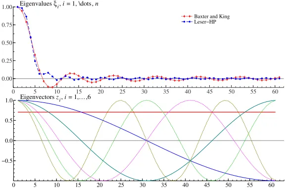
Figure 1: Eigen-decomposition of the smoothing matrices corresponding to the Baxter and King low-pass filter with cutoff frequency corresponding to 10 years (quarterly data) and to the Leser-Hodrick-Prescott filter with smoothing parameter 1600.
0 5 10 15 20 25 30 35 40 45 50 55 60
0.00 0.25 0.50 0.75
1.00 Eigenvalues ξi, i = 1, \dots, n
Baxter and King Leser−HP
0 5 10 15 20 25 30 35 40 45 50 55 60
−0.5 0.0 0.5
1.0 Eigenvectors zi, i = 1,…,6
The results of the preceding sections can also be relevant for the desing of a filter in the time domain. The method consists of modifyingS so thatn−k high frequency noisy components receive zero weight. This is done through the spectral decomposition ofH.
Decomposing S = H+∆H andH = ZXZ′, whereX = diag{ξ
1, ξ2, ..., ξn}, and writing
y=Zθ, we get
Sy = ZXθ+∆HZθ
≈ ZXkθ+∆HZθ
where Xk is the matrix obtained by replacing with zeros the eigenvalues ofHthat are smaller than a cut-off eigenvalueξkand∆HZθ is a null vector except for the first and last elements that
account for the boundary conditions. Turning to the original coordinate system and arranging the boundaries, we get the new estimator
Sk = Hk+∆k+∆H
= H(k)+∆H
whereH(k) is the matrix with boundaries equal to those ofHand interior equal to that ofHk =
ZXkZ′. In other words,H(k) is structured like (2) withHak =Ha,Hak∗ =EhHaEh andHsk =
[ZXkZ′]s. Hence a new smoothing matrix is obtained,Sk, and consequently new trend estimates, saymˆk.
In practice, the procedure is very easy to apply. In fact, given a symmetric filter, it consists of: obtainingH, replacing it byHkand then adjusting the boundaries with suitable chosen asymmet-ric filters to getSk.
4
Appendix: proof of Theorem 1
Let us writeS=H+∆H. The matrixHis diagonalised by the orthogonal matrix
Z=
r
2
n
·
kjcos
(2i−1)(j−1)π
2n
¸
ij
, i, j = 1,2, ..., n
wherekj = √12 forj = 1andkj = 1forj >1which satisfieskZk2kZ−1k2 = 1. The spectrum
ofHisσ(H) ={ξ1, ξ2, ..., ξn}, where
ξi= n
X
j=1 µ
2 cos(i−1)π
n
¶j−1
cj
which follows by (3) and by the fact that the eigenvalues ofT11are (Bini and Capovani, 1983)
ϑi = 2 cos
(i−1)π n .
Setting δH = k∆Hk2 and applying the Bauer-Fike theorem (Bauer and Fike, 1960) with the
2-norm as an absolute norm gives
¯ ¯ ¯ ¯ ¯ ¯ λ− n X j=1 µ
2 cos(i−1)π
n
¶j−1
cj ¯ ¯ ¯ ¯ ¯ ¯
≤δH.
We now prove thatcj = 0forj > m+ 1, so that the above summation involves justm+ 1 terms instead ofn. It follows by the Cramer rule that, explicitly,
cj =
detQ[j,h] detQ
whereQ[j,h]is the matrix obtained replacing thej-th column ofQby the vectorh. The matrix
Qis upper triangular with ones on the diagonal so its its determinant is equal to one and since the generic elementhj ofhis null forj > m+ 1it follows thatdetQ[j,h] = 0andcj will be null as well.
Finally, we prove that
cj =wj−1+
⌊m−j−1 2 ⌋
X
q=0
(−1)q+1(j)
q
(q+ 1)! (j+ 2q+ 1)wj+2q+1. (8)
This expression can be directly verified by calculatingdetQ[j,h]for allj. Here in the following, we prove it by induction overj= 1, ..., m+ 1, withm∈N.
• For j = 1, c1 = w0+P m−2
2
q=0 (−1)q+12w2q+2 which follows by(1)q = q!and by simple algebra. The linear system Qc = h can be written as c = Q−1(h
1 +h2) with h1 =
[w0,w1, ...,wm,0, ...,0]′ andh2 = [w1,w2, ...,wm,0, ...,0]′, bothn-dimensional vectors. Since the first row of Q−1 is the vector [1,−1,−1,1,1,−1,−1, ...]we have that c
1 =
(w0+w1)−(w1+w2)−(w2+w3) + (w2+w4) +...+ (−1)⌊ m−2
2 ⌋+12w
2⌊m−2 2 ⌋+2
• Forj=m,cm =wm−1as it is immediate to see given that the summation inqwas defined
for non negative values of m−2j−1. All the more so, it implies thatcm+1 = wm. Hence
we have showed that (8) holds forj = 1 and that, if it holds forj = m then it holds for
j =m+ 1. This proves that (8) is true for allm∈N. The proof of theorem 2 is therefore
complete¥
Acknowledgements
We would like to kindly thank Dario Bini for the valuable suggestions and discussions.
References
Bauer F., Fike C. (1960), Norms and Exclusion Theorems, Numerische Mathematik, 2, 137-141.
Baxter, M., King, R.G. (1999). Measuring Business Cycles: Approximate Band-Pass Filters for Economic Time Series.The Review of Economics and Statistics, 81, 575593.
Bini D., Capovani M. (1983), Spectral and computational properties of band symmetric Toeplitz matrices,Linear Algebra and its Applications, 52/53, pp. 99-126 .
Bini D., Favati P. (1993), On a matrix algebra related to the discrete Hartley transform. SIMAX, 14, 2, 500-507
B¨ottcher A., Grudsky, S.M. (2005),Spectral Properties of Banded Toeplitz Matrices, Siam.
Bozzo E., Di Fiore C. (1995), On the use of certain matrix algebras associated with discrete trigonometric transforms in matrix displacement decomposition,Siam J. Matrix anal. Appl., 16, 1, 312-326.
Buja A., Hastie T.J., Tibshirani R.J.(1989), Linear Smoothers and Additive Models,The Annals of Statistics, 17, 2, 453-555.
Christiano L.J., Fitzgerald T.J., (2003), The band pass filter,International Economic Review, 44, 435-465.
Cleveland, W.S., Loader, C.L. (1996). Smoothing by Local Regression: Principles and Meth-ods. In W. H¨ardle and M. G. Schimek, editors,Statistical Theory and Computational As-pects of Smoothing, 1049. Springer, New York.
Dagum, E.B., Luati, A. (2004). A Linear Transformation and its Properties with Special Ap-plications in Time Series,Linear Algebra and its Applications, 338, 107-117.
Davis, P.J., (1979).Circulant matrices, Wiley, New York.
Fan J. and Gjibels I. (1996). Local Polynomial Modelling and its Applications, Chapman and Hall, New York.
Gray R.M. (2006)Toeplitz and Circulant Matrices: A review, Foundations and Trends in Com-munications and Information Theory, Vol 2, Issue 3, pp 155-239.
Green P.J. and Silverman, B.V. (1994) Nonparametric Regression and Generalized Linear Models: a Roughness Penalty Approach. Chapman & Hall, London.
Grenander, U., Szeg¨o, G. (1958). Toeplitz Forms and Their Applications, University of Cali-fornia Press.
Hastie T.J. and Tibshirani R.J.(1990),Generalized Additive Models, Chapman and Hall, Lon-don.
Hodrick, R., and Prescott, E.C. (1997). Postwar U.S. Business Cycle: an Empirical Investiga-tion,Journal of Money, Credit and Banking, 29, 1, 1-16.
Kailath T., Sayed A. (1995) Displacement Structure: Theory and Applications,SIAM Review, 37, 3, 297-386.
Leser, C.E.V. (1961). A Simple Method of Trend Construction,Journal of the Royal Statistical Society B, 23, 91-107.
Percival, D.B., Walden, A.T. (2000). Wavelet Methods for Time Series Analysis. Cambridge Se-ries in Statistical and Probabilistic Mathematics. Cambridge University Press, Cambridge.
Pollock, D.S.G. (2002), Circulant matrices and time-series analysis,International Journal of Mathematical Education in Science and Technology, 33, 2, 1, 213-230(18)
Proietti, T., Luati, A. (2009). Real Time Estimation in Local Polynomial Regression, with an Application to Trend-Cycle Analysis,Annals of Applied Statistics, forthcoming.
Ruppert D., Wand, M.J., Carroll R.J. (2003). Semiparametric regression, Cambridge Univer-sity Press.
Weaver J.R. (1985), Centrosymmetric (Cross-Symmetric) Matrices, their Basic Properties, Eigenvalues, Eigenvectors,Amer. Math. Monthly, 92, 711-717.