Published Online January 2014
Real-Time Short-Term Forecasting Based
on Information Management
Jamal Raiyn1, Tomer Toledo2
1
Faculty of Exact Science, Computer Science Department, Al Qasemi Acedemic College,Haifa, Israel
2
Faculty of Civil and Environmental Engineering, Department of Transportation Engineering, Technion-Israel Institute of Technology, Haifa, Israel
Email:
Received August 11, 2013; revised September 12; 2013; accepted October 9, 2013
Copyright © 2014 Jamal Raiyn, Tomer Toledo. This is an open access article distributed under the Creative Commons Attribution License, which permits unrestricted use, distribution, and reproduction in any medium, provided the original work is properly cited. In accordance of the Creative Commons Attribution License all Copyrights © 2014 are reserved for SCIRP and the owner of the intellectual property Jamal Raiyn, Tomer Toledo. All Copyright © 2014 are guarded by law and by SCIRP as a guardian.
ABSTRACT
Traffic congestions and road accidents continue to increase in industry countries. There are three basic strate-gies to relieve congestion. The first strategy is to increase the transportation infrastructure. However, this strat-egy is very expensive and can only be accomplished in the long-term. The second stratstrat-egy is to limit the traffic demand or make traveling more expensive that will be strongly opposed by travelers. The third strategy is to focus on efficient and intelligent utilization of the existing transportation infrastructures. This strategy is gaining more and more attention because it’s well. Currently, the Intelligent Transportation System (ITS) is the most promising approach to implementing the third strategy. Various forecast schemes have been proposed to manage the traffic data. Many studies showed that the moving average schemes offered meaningful results compared to different forecast schemes. This paper considered the moving average schemes, namely, simple moving average, weighted moving average, and exponential moving average. Furthermore, the performance analysis of the short- term forecast schemes will be discussed. Moreover, the real-time forecast model will consider the abnormal con- dition detection.
KEYWORDS
Forecast Scheme; Moving Average; Intelligent Transportation System
1. Introduction
This paper introduces a modern forecast strategy. Con-ceptually, traffic information [1,2] may fall into one of the three categories as follows: historical information, real-time information, and predictive information. The historical data [3,4] are a collection of past observations of the system. Real-time information is the most up-to- date and can be calculated, e.g., by on-line simulations. The real-time information achieves to update the histori-cal adaptive information, special in the case that the real- time information does not match the historical informa-tion. To optimize the forecast algorithm, we have col-lected travel data by the mobile phone. For a successful forecast of traffic flow, it ought to apperceive the variety of environment and can adjust the parameters automati-cally. Furthermore, it is important that the forecast model
takes into consideration the abnormal conditions that occurred in real-time [5,6]. The paper is organized as follows. Section 2 describes the problem in transporta-tion engineering. Sectransporta-tion 3 introduces the informatransporta-tion collection based on cellular phone services. Section 4 introduces the short-term forecast scheme based on his-torical and real-time information. Section 5 discusses the performance analysis of the proposed short-term forecast scheme based on exponential moving average.
2. Methodology
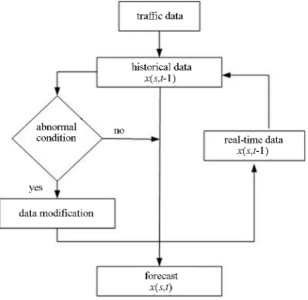
data collection technologies and data processing algo-rithms. Variations in cellular mobile services [7] and algorithm schemes result in a variety of solutions for incident detection. Various short-term traffic forecasting scheme have been proposed [8-19]. In this section we introduce the forecast model based on the moving aver-age. There are three types of moving average, that is, simple moving average (SMA), weight moving average (WMA), and exponential moving average (EMA) [20- 23]. In this study, an exponential moving average is con-sidered. An exponential moving average uses a weight- ing or a smoothing factor which decreases exponentially. The weighting for each older data point decreases ex- ponentially, giving much more importance to recent ob- servations while not discarding the older observations entirely. Figure 1 illustrated the proposed forecast model. The forecast model is divided into two phases, namely, detection phase, and forecast phase. The detection phase focused on the collected data analysis. To increase the accuracy of the forecast model we need to detect the ab-normal events in the collected data. The forecast scheme is based on the exponential moving average. The robust-ness and accuracy of the exponential smoothing fore- cast is high and impressive. The accuracy of the expo-nential smoothing technique depends on the weight smoothed factor alpha value of the current demand. To determine the optimal alpha factor value we use the fit-ting curve.
[image:2.595.62.287.501.720.2]There are two kinds of exponential moving average forecasting (EMA) that is exponential moving average based historical information (EMA-H) and exponential moving average based real-time information (EMA-R). The EMA-R consists of two main phases, namely detec-
Figure 1. Algorithm process.
tion phase and forecast phase
2.1. Forecast Based Historic Observations
The historical database is a collection of past travel ob-servations of the system. Exponential smoothing is fore-casting method that gives weight to the observed time series unequally. The unequal weight is accomplished by using one or more smoothing parameters, which deter-mine how much weight is given to each observation. The major advantage of exponential smoothing methods is that gives good forecasts in a wide variety of applications. In addition, data storage and computing requirements are minimal, which makes exponential smoothing suitable for real-time application.
(
1,)
M( ) (
, 1)
H( )
,tt t+ k = ∗α tt t k + −α ∗tt t k (1)
where 0< ≤α 1, M
( )
,tt t k the actual travel time in
section k at the time H
( )
,t tt⋅ t k the historical travel time in section k at time t.
Smoothed Parameter Alpha
To achieve short-term traffic flow forecasting with high accuracy, the proposed forecast scheme required to op-
timize the smoothed parameter alpha. Alphadetermines
how responsive a forecast is to sudden jumps and drops. It is the percentage weight given to the prior, and the remainder is distributed to the other historical periods. Alpha is used in all exponential smoothing methods. The lower the value of alpha, the less responsive the forecast is to sudden change. The smoothing parameter “alpha” lies between 0 and 1. To determine the optimized smoothing factor, a sum of the square errors between the observed and the forecasted alpha dose rates was ana-lyzed by increasing the smoothing filter factor from 0.1. Sum of the square errors is decreased as the smoothing filter factor is increased as showed in Figure 2.
Figure 2. Smoothed parameter alpha.
0.1 0.2 0.3 0.4 0.5 0.6 0.7 0.8 0.9 1 83.6
83.8 84 84.2 84.4 84.6 84.8 85 85.2 85.4 85.6
alpha
[image:2.595.309.535.535.717.2]13
2.2. Real-Time Forecasting
Occurrence of Abnormal conditions in flow travel infor-mation decrease the accuracy of the forecasting based historical information and may increase the complexity of the forecasting of unusual incidence. The forecast model in real-time gives a small weight to the history information and a big weight to the real-time observa- tion.
(
1,)
H(
1,)
(
M( )
, H( )
,)
tt t+ k =tt t+ k + ∗γ tt t k −tt t k
(2) where 0< <γ 1.
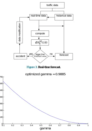
Figure 3 illustrates the real-time forecast model in abnormal conditions.
[image:3.595.158.453.302.722.2]2.2.1. Smoothed Parameter-Gamma
Figure 4illustrated that the value of gamma for real-time
forecasting is closed to 0.9885.
2.2.2. Section Mutual Influence
In the real-time forecasting we take into consideration the effect of the upstream (UP) and downstream (DS).
(
)
(
)
12 3
1, H 1, desired
tt t k tt t k
UP DS
γ
γ γ
+ = + + ∗
+ ∗ + ∗ (3)
where
( )
( )
desired=ttM t k, −ttH t k,
(
)
(
)
upstearm=ttM t k, − −1 ttH t k, −1
(
)
(
)
downstream=ttM t k, + −1 ttH t k, +1
k is the desired section,
(
k−1)
is the upstream section(
k+1)
is the downstream section.traffic data
historical data real-time data
forecast
data modification
compute
bigger than
threshold value
accident
)) , ( (ttkM tk σ
no yes
[image:3.595.205.393.309.507.2]Figure 3. Real-time forecast.
Figure 4. Smoothed parameter gamma.
0.1 0.2 0.3 0.4 0.5 0.6 0.7 0.8 0.9 1 0
100 200 300 400 500 600 700
gamma
2.3. Accident Detection Strategy
The performance of an incident detection system is de- termined on two levels: data collection and data proces- sing. Data collection refers to the detection/sense/sur- veillance technologies that are used to obtain traffic flow data. Data processing refers to the algorithms used for detecting and classifying incidents through analyzing the traffic parameters from detectors or sensors for the pur- pose of alerting observers of the occurrence, severity, and location of an incident. The hybrid of data collection strategies and data processing methodologies results in a variety of solutions for incident detection. The main task of the proposed accident detection (AD) algorithm is to identify and distinguish different traffic modes. It de- pends on an upstream occupation increase and a down- stream occupation decrease at the level of loop detector where an incident happened. This algorithm compares a value of a traffic flow parameter with a known value. The algorithm trusts that an upstream occupation will increase and downstream occupation will decrease where an incident happened. In traffic incident detection, a time sequence is used to describe a traffic state. When a cur- rent measured value is deviated from the output of the algorithm seriously, the algorithm will think that an in-cident has occurred. The time sequence analytic algo- rithms include a moving average algorithm, an exponen- tial smoothing algorithm.
● The accident characterized by temporal variation of
speed at fixed road section (location) that expressed as the coefficient of variation in speed.
● The spatial variation of speed along road sections
expressed as the difference in speed between up- stream and downstream location (Q).
( )
, 1(
, 2)
Q= tt t s −tt t s (4)
where tt t s
(
, 1)
, tt t s(
, 2)
average speeds computedover period of t upstream and downstream of a road
sections, respectively (km/h).
2.3.1. Incident-Influence Traffic Data
An incident occurring on section i within time interval
t is considered to have a significant impact on traffic when traffic measurements from the upstream and down-stream stations satisfy the following conditions:
1) The difference between upstream speed si t , and downstream speed si+1, t is greater than the thre-shold value;
2) The ratio of the difference between the upstream and downstream speeds to the upstream speed
(
si t, − +si 1,t)
si t, , is greater than the threshold value; and3) The ratio of the difference between the upstream and downstream speeds to the downstream speed
(
si t, − +si 1,t)
si+1,t is greater than the threshold val-ue.
The abnormal record shows that at least 30 km/h lower traffic speed than the average speed of all records at the same time on the same day of the week. The threshold of 30km/h is a symbolic value of the smallest speed change that people would consider “abnormal”. The vehicle speed starts to decrease in upstream however the speed in downstream starts to increase.
( ) (
)
( )
, 1,
threshold ,
tt k t tt k t
tt k t
− +
> (5)
( , ) ( 1, )
threshold
( 1, )
tt k t tt k t tt k t
− + >
+ (6)
2.3.2. Real-Time Accident Detection
The travel time forecast model considers the incident and non-incident conditions. We make different between ● Accident during peak time (morning/afternoon) ● Accident during regular time
● Heavy accident
● Light accident
The accident is cleared at current time t in section s, the duration is known and the speed is considered to be 30 km reduced of the average speed.
(
1,)
H(
1,)
( )
(
tM tH)
t
tt t+ k =tt t+ k + ∗γ P ∗ tt −tt (7)
(
)
1accident
1 t
t t
P P
e−υ
= =
+ ,
1 1 2 2 3 3 4 4
t x x x x
υ =β +β +β +β
(
)
(
)
1 , 2
H H
t t t t
H H
t t
tt tt
x σ σ x
σ σ
− −
= = ,
(
) (
1 1)
3
1
H H
t t t t
H H
t t
tt tt tt tt x σ σ − − − − − = − ,
(
) (
1 1)
4
1
H H
t t t t
H H
t t
x σ σ σ σ
σ σ
− −
−
− −
= −
where X denotes the vector of predictor variables. β is the vector of coefficient associated with the predictor va0 riables. and can be computed according to the binary logit model. νt is the logit link function (which is a linear combination of the predictor variables).
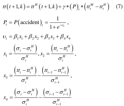
2.4. Smoothed Parameter Optimization
To increase the exponential moving average forecast accuracy in real-time, the smoothed parameter alpha and
gamma in Equation (2) should be optimized. Figure 5
[image:4.595.324.541.385.570.2]illustrated the value of the optimized smoothed parameter gamma in real-time accident conditions.
15
Figure 5. Gamma value AD.
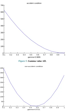
Figure 6. Gamma value in NAD.
parameter gamma in real-timenon-accident conditions. Based on Equation (7), the optimized parameters in real-timeaccident conditions and real-time non-accident conditions are summarized in Table 1.
3. Performance Analysis
There are various measures of forecasting accuracy tech-niques proposed in the literature [24-29]. The aim of this study is to evaluate forecast accuracy travel observations. The forecasting accuracy techniques are used to be able to select the most accurate forecast scheme. Furthermore we aim to analyze the moving average schemes, namely simple moving average, weighted moving average, and exponential moving average. The forecasting perfor- mance of the various models and the measures of the predictive effectiveness was evaluated using various
summary statistics. The comparing experiments are car-ried out under normal traffic condition and abnormal traffic condition to evaluate the performance of four main branches of forecasting models on direct travel time data obtained by license plate matching (LPM). The MAE is a measure of overall accuracy that gives an in- dication of the degree of spread, where all errors are as- signed equal weights. The MSE is also a measure of overall accuracy that gives an indication of the degree of spread, but here large errors are given additional weight. It is the most common measure of forecasting accuracy. Often the square root of the MSE, RMSE, is considered, since the seriousness of the forecast error is then denoted in the same dimensions as the actual and forecast values themselves. Mean square percentage error (MSPE) is the relative measure that corresponds to the MSE. The more
0.1 0.2 0.3 0.4 0.5 0.6 0.7 0.8 0.9 1
0 100 200 300 400 500 600 700
gamma=0.9895 accident condition
0.1 0.2 0.3 0.4 0.5 0.6 0.7 0.8 0.9 1 0
50 100 150 200 250 300 350 400
commonly used measure is the root mean square percen-tage error (RMSPE). Theil’s Coefficient is another statis- tical measure of forecast accuracy. One specification of theil’s compares the accuracy of a forecast model to that of a naïve model. A theil’s greater than 1.0 indicates that the forecast model is worse than the naïve model; a val- ues less than 1.0 indicates that it is better. The closer U is to 0, the better the model.
Modern vs. Traditional Traffic Data
In this section we illustrate the simulation results and analysis of the implementation of the measured traffic speeds and travel time. The information of the dual magnet loop detectors will be compared to the informa- tion that is provided from cellular phone service. Based on the WEKA platform we have carry out analysis and comparison of different Prediction schemes. WEKA (Waikato Environment for Knowledge Analysis) is a col- lection of machine learning algorithms for data mining tasks. WEKA contains tools for data pre-processing, classification, regression, clustering, association rules and visualization [30]. We have used the WEKA to make comparison between the following schemes:
1) Smoothed Linear Models (LM) 2) Tree Decision (TD)
3) Nearest- Neighbor Classifier (NN)
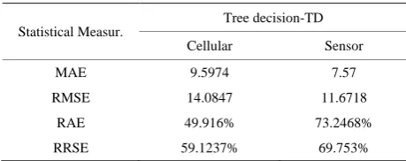
The comparison is focused on various statistical mea-surements error, mean absolute error (MAE), root mean squared error (RMSE), relative absolute error (RAE), root relative squared error (RRSE), and Theil’s coeffi-cient. Tables 2-4 illustrate general comparison between cellular travel speed and sensor travel speed. The results
of the quality measurements are summarized in Tables
2-4. Furthermore Tables 2-4 illustrate that the Nearest
Table 1. Optimized parameters in AD/NAD.
AD no AD
γ 0.9993 0.5346
1
β 1.0004 0.2215
2
β 1.0018 0.1138
3
β 0.9998 0.2315
4
β 0.9993 0.4643
Table 2. Cellular vs. sensor based on LM.
Statistical Measur.
Linear model-LM
Cellular Sensor
MAE 7.973 7.1967
RMSE 11.6976 11.5308
RAE 41.4674% 69.6342%
RRSE 49.1034% 68.9102%
[image:6.595.307.537.425.516.2]Neighbor Scheme offers a clear and the best results compared to the linear model and tree decision schemes.
Table 5 illustrates a comparison between the SMA, WMA, EMA.
4. Simulation Results
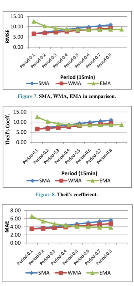
Results indicate that all three moving average methods, SMA, WMA and EMA, have more or less similar per-formance in forecasting short-term travel times. However, as one would expect the method using optimized weights produced slightly better forecasts at a higher computa-tional cost. Quality of forecasts is diminished as the time for which forecasts are made is farther in the future. Moving average methods overestimate travel speeds in slow-downs and underestimate them when the conges-tion is clearing up and speeds are increasing. Figures 7-9
described the comparison between SMA, WMA and EMA based on the various statistical measurements error.
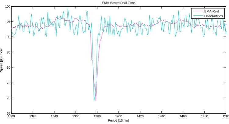
Figure 10 compared the EMA to optimized EMA based on historical observations. Figures 11 and12 showed the actual observations compared to EMA based Information and to EMA based on real-time information. Results in-dicate that all three moving average methods have more or less similar performance in forecasting short-term tra-vel times. However, as one would expect the method using optimized weights produced slightly better fore-
Table 3. Cellular vs. sensor based on TD.
Statistical Measur.
Tree decision-TD
Cellular Sensor
MAE 9.5974 7.57
RMSE 14.0847 11.6718
RAE 49.916% 73.2468%
[image:6.595.308.539.545.634.2]RRSE 59.1237% 69.753%
Table 4. Cellular vs. sensor based on NN.
Statistical Measur.
Nearest Neighbour
Cellular Sensor
MAE 6.4734 6.6224
RMSE 10.1594 11.0445
RAE 33.6678% 64.0777%
[image:6.595.308.538.662.734.2]RRSE 42.6465% 66.0042%
Table 5. SMA vs. WMA vs. EMA.
statistical Measurements SMA WMA EMA
MAE 6.22 8.11 5.17
RMSE 12.33 14.04 9.57
RAE 11.84 16.54 11.54
Theil’s Coefficient 7.21 9.55 5.61
17
Figure 7. SMA, WMA, EMA in comparison.
Figure 8. Theil’s coefficient.
Figure 9. MAE.
casts at a higher computational cost. Quality of forecast is diminished as the time for which forecasts are made is farther in the future. Moving average methods overesti-mate travel speeds in slow-downs and underestioveresti-mate them when the congestion is clearing up and speeds are increasing. Figure 13illustrated the comparison between the exponential moving average based historical infor-mation (EMA-H) and the exponential moving average based real-time information (EMA-R) compared to ac-tual observations. EMA-H detects the abnormal condi-tions in travel flow traffic based pervious information that are collected in same location and at the same time. The advantage of the EMA-H is an identification of in-
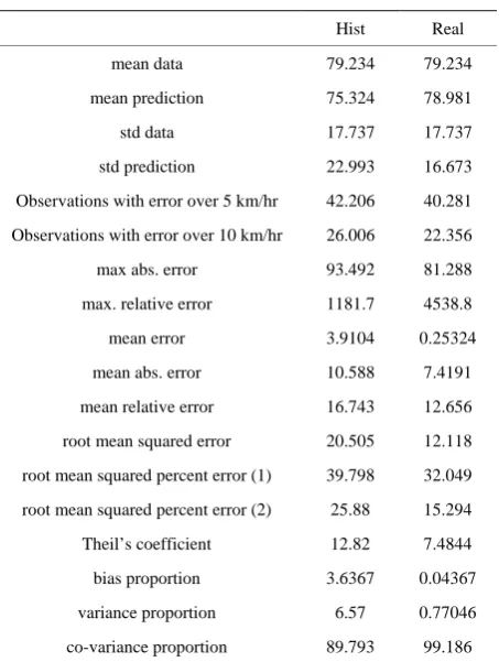
cident in flow traffic. However a repeated incident with the same characteristics in the future is not certain. Fur-thermore Figure 13 illustrated that EMA-R identify the incident in the flow traffic and provides incident clear-ness. Tables 6 and7illustrated the comparison between EMA based historical information and EMA based real- time in accident and in non accident conditions.
5. Conclusion
Figure 10. Comparison between EMA and Opt-EMA.
Figure 11. EMA-H vs. actual observations.
Figure 12. EMA-R vs. actual observations.
1200 1250 1300 1350 1400 1450 1500 1550 1600 60
65 70 75 80 85 90 95 100 105
Period [15min]
S
peed [
km
/hour
]
EMA Based Historic
EMA-Historic Observations
1300 1320 1340 1360 1380 1400 1420 1440 1460 1480 1500
65 70 75 80 85 90 95 100
Period [15min]
S
peed [
]k
m
/hour
EMA Based Real-Time
[image:8.595.110.486.509.713.2]19
Figure 13. EMA-H, EMA-R in comparison.
Table 6. Historical vs. real-time in AD.
Hist Real
mean data 79.234 79.234
mean prediction 75.324 78.981
std data 17.737 17.737
std prediction 22.993 16.673
Observations with error over 5 km/hr 42.206 40.281
Observations with error over 10 km/hr 26.006 22.356
max abs. error 93.492 81.288
max. relative error 1181.7 4538.8
mean error 3.9104 0.25324
mean abs. error 10.588 7.4191
mean relative error 16.743 12.656
root mean squared error 20.505 12.118
root mean squared percent error (1) 39.798 32.049
root mean squared percent error (2) 25.88 15.294
Theil’s coefficient 12.82 7.4844
bias proportion 3.6367 0.04367
variance proportion 6.57 0.77046
co-variance proportion 89.793 99.186
[image:9.595.61.288.336.637.2]different forecast schemes. In this paper, we have intro-duced various forecast schemes based on the historical data and real-time observations. Furthermore, in this pa-per, we discuss and summarize some prediction methods based on their performance analysis. We conclude that the optimized exponential moving average is the most accu-rate method. Moreover, the proposed algorithm has been
Table 7. Historical vs. real-time in NAD.
Hist Real
mean data 67.805 67.805
mean prediction 65.622 66.798
std data 17.809 17.809
std prediction 18.682 16.968
Observations with error over 5 km/hr 33.086 31.293
Observations with error over 10 km/hr 17.385 15.735
max abs. error 73.39 73.264
max. relative error 587.12 586.11
mean error 2.183 1.0076
mean abs. error 6.6768 5.472
mean relative error 12.238 10.562
root mean squared error 12.452 9.2418
root mean squared percent error (1) 26.42 23.514
root mean squared percent error (2) 18.364 13.63
Theil’'s coefficient 9.0011 6.6476
bias proportion 3.0737 1.1886
variance proportion 0.49122 0.82716
co-variance proportion 96.435 97.984
given the best solution for traffic travel forecast. However, the number of the road accidents increase rapidly. To re- duce the incidents, a new detection scheme should be dev- eloped that takes driver’s behaviors into consideration.
REFERENCES
[1] J. P. Bickel, C. Chen, J. Kwon, J. Rice, V. E. Zwet and P. Varaiya, “Measuring Traffic,” Statistical Science, Vol. 22,
1300 1320 1340 1360 1380 1400 1420 1440 1460 1480 1500
60 65 70 75 80 85 90 95 100
Period [15min]
S
peed [
k
m
/hour
]
EMA-Historic vs EMA-Real
[image:9.595.304.541.339.618.2]No. 4, 2007, pp. 581-597.
[2] T. M. Borzacchielo, “The Use of Data from Mobile Phone Networks for Transportation Applications,” Tran- sportation Research Board, 2010, 20 p.
[3] R. Chrobok, O. Kaumann, J. Wahle and M. Scheckenberg, “Three Categories of Traffic Data: Historical, Current, and Predictive,” 9th IFAC Symposium, Braunschweig, Vol. 1, 13-15 June 2000, pp. 221-226.
[4] R. Chrobok, O. Kaumann, J. Wahle and M. Schrecken- berg, “Different Methods of Traffic Forecast Based on Real Data,” European Journal of Operational Research, Vol. 15, No. 3, 2004, pp. 558-568.
[5] M. Alger, “Real-Time Traffic Monitoring Using Mobile Phone Data,” Proceedings on 49th European Study, 2004. [6] D. Wild, “Short-Term Forecasting Based on a Transfor- mation and Classification of Traffic Volume Time Series,” International Journal of Forecasting, Vol. 13. No. 1, 1997, pp. 63-72.
[7] Y. Lv and S. Tang, “Real-Time Highway Traffic Acci- dent Prediction Based on the k-Nearest Neighbor Method,” International Conference on Measuring Technology and Mechatronics Automation, Vol. 3, 2010, pp. 547-550. [8] Y. Lee and C. H. Wei, “A Computerized Feature Selec-
tion Using Genetic Algorithms to Forecast Freeway Ac- cident Duration Times,” Computer-Aided Civil and Infra- structure Engineering, Vol. 25, No. 2, 2010, pp. 132-148.
[9] M. Martínez-Zarzuela, “Wavelet-Based Denoising for Traffic Volume Time Series Forecasting with Self-Or- ganizing Neural Networks,” Computer-Aided Civil and Infrastructure Engineering, Vol. 25, No. 7, 2010, p. 530- 545.
[10] H. Nicholson and C. D. Swann, “The Prediction of Traf- fic Flow Volumes Based on Spectral Analysis,” Trans- portation Research, Vol. 8, No. 6, 1974, pp. 533-538.
[11] I. Okutani and J. Y. Stephanedes, “Dynamic Prediction of Traffic Volume through Kalman Filtering Theory,” Tran- sportation Research, Vol. 18B, No. 1, 1984, pp. 1-11.
[12] B. Ronen, A. Coman and E. Schragenheim, “Peak Man- agement,” International Journal of Production Research, Vol. 39, No. 14, 2011, pp. 3183-3193.
[13] M. Sabry, H. Abd-El-Latif, S. Yousef and N. Badra, “A Time-Series Forecasting of Average Daily Traffic Vo- lume,” Australian Journal of Basic and Applied Sciences, Vol. 1, No. 4, 2007, pp. 386-394.
[14] M. Sabry, H. Abd-El-Latif and N. Badra, “Comparison between Regression and Arima Models in Forecasting Traffic Volume,” Australian Journal of Basic and Appli- ed Sciences, Vol. 1, No. 2, 2007, pp. 126-136.
[15] A. Stathopoulos, L. Dimitriou and T. Tsekeris, “Fuzzy Modeling Approach for Combined Forecasting of Urban Traffic Flow,” Computer-Aided Civil and Infrastructure
Engineering, Vol. 23, No. 7, 2008, pp. 521-535.
[16] Y. J. Stephanedes, P. G. Michalopoulos and R. A. Plum, “Improved Estimation of Traffic Flow for Real-Time Control,” Transportation Research Record, Vol. 795, 1981, pp. 28-39.
[17] H. Tu, H. Van Lint and H. Van Zuylen, “The Effects of Traffic Accidents on Travel Time Reliability,” IEEE Conference on Intelligent Transportation Systems, Bei- jing, 12-15 October 2008, pp. 79-84.
[18] E. I. Vlahogianni, M. G. Karlaftis and J. C. Golias, “Tem- poral Evolution of Short-Term Urban Traffic Flow: A Non-Linear Dynamics Approach,” Computer-Aided Civil and Infrastructure Engineering, Vol. 23, No. 7, 2008, pp. 536-548.
[19] Z. Wang and P. Murray-Tuite, “Modeling Incident-Relat- ed Traffic and Estimating Travel Time with a Cellular Automaton Model,” Transportation Research Board, 2010, 21 p.
[20] M. S. Ahmed and A. R. Cook, “Analysis of Freeway Traffic Time-Series Data by Using Box-Jenkins Techni- ques,” Transportation Research Record, Vol. 722, 1997, pp. 1-9.
[21] J. Andrada-Felix and F. Fernandez-Rodriguez, “Improv- ing Moving Average Trading Rules with Boosting and Statistical Learning Methods,” Journal of Forecasting, Vol. 27, No. 5, 2008, pp. 433-449.
[22] R. R. Andrawis and F. A. Atiya, “A New Bayesian For- mulation for Holt’s Exponential Smoothing,” Journal of Forecasting, Vol. 28, No. 3, 2009, pp. 218-234.
[23] A. Guin, “Travel Time Prediction using a Seasonal Auto- regressive Integrated Moving Average Time Series Mod- el,” Proceedings of the IEEE Intelligent Transportation Systems Conference, Toronto, 17-20 September 2006, pp. 493-498.
[24] H. Jo, B. Lee, Y.-C. Na, H. Lee and B. Oh, “Prioritized Traffic Information Delivery Based on Historical Data Analysis,” Proceedings of the 2007 IEEE Intelligence Transportation Systems Conference, Seattle, 30 Septem- ber-3 October 2007, pp. 568-573.
[25] A. Karim and H. Adeli, “Fast Automatic Incident Detec- tion on Urban and Rural Freeways Using Wavelet Energy Algorithm,” Journal of Transportation Engineering, ASCE, Vol. 129, No. 1, 2003, pp. 57-68.
[26] H. Lee, N. K. Chowdhury and J. Chang, “A New Travel Time Prediction Method for Intelligent Transportation Systems,” Springer-Verlag, Berlin, 2008, pp. 473-483. [27] J. Xia, “Predicting Freeway Travel Time Under Incident
Condition,” Transportation Research Record: Journal of the Transportation Research Board, 2010, pp. 58-66. [28] X. Q. Zhao, R. M. Li and X. X. Yu, “Incident Duration
21
ligent Computation Technology and Automation, Chang- sha, 10-11 October 2009, pp. 625-628.
[29] X. Zheng and M. Liu, “An Overview of Accident Fore- casting Methodologies,” Journal of Loss Prevention in the Process Industries, Vol. 22, No. 4, 2009, pp. 484-491.