Closed form approximations to the Error and Complementary Error Functions and their applications in atmospheric science

Title:

Closed-form approximations to the Error and Complementary Error Functions and their applications in atmospheric science

Short title:

Closed-form of Error and Complementary Error Functions Authors:

C. Ren and A. R. MacKenzie Affiliation:

Department of Environmental Sciences Lancaster University,

Lancaster LA1 4YQ United Kingdom

Corresponding author: C. Ren

Address:

Department of Environmental Sciences Lancaster University,

Lancaster LA1 4YQ United Kingdom

E-mail: [email protected]. Tel: +44-1524-593974

Abstract

The Error function, and related functions, occurs in

theoretical aspects of many parts of atmospheric science. This note presents a closed-form approximation for the error,

complementary error, and scaled complementary error functions, with maximum relative errors within 0.8%. Unlike other approximate solutions, this single equation gives answers within the stated accuracy for x∈

[

0 ∞

)

. The approximation is very useful in solving atmospheric science problems by providing analytical solutions. Examples of the utility of the approximations are: the computation of cirrus cloud physics inside a general circulation model, the cumulative distribution functions of normal and log-normal

distributions, and the recurrence period for risk assessment. Keyword

Error function, complementary error function, scaled complementary error function, normal distribution, log-normal distribution,

cumulative distribution function, recurrence interval Introduction

Error and complementary error functions are extensively used in the fields that employ mathematics and physics, e.g., studies of heat and mass transfer (e.g., Chaudhry and Zubair, 1993;

Swartzendruber, 2002). In atmospheric science, as elsewhere, the error and complementary error functions occur when normal or log-normal distributions are expressed as cumulative distribution functions. This note presents a close-form approximation for the error, complementary error, and scaled complementary error

functions with maximum relative errors within 0.8%. The benefits of using an analytical approximation for error function in

atmospheric sciences are demonstrated in some examples. The closed-form approximation of error functions

The error function is defined as

( )

₌

_∫

x − t

dt e x

erf

0

2 2

π , (1)

and the complementary error function is defined as

( )

_{≡ −}

( )

₌

_∫

∞ −

x t

dt e x

erf x

erfc 1 2 2

π . (2)

Both functions contain integrals. Sometimes, when one wants to evaluate these functions as accurately as possible, rational Chebyshev approximations (Cody, 1969) can be used. Nowadays, built-in functions are available in several computer languages (Cody, 1990). At other times, however, one may forego some

quick to compute, but all fail to give expressions in closed form. The following achieves closed-form approximations for the error, complementary error, and scaled complementary error functions with maximum relative errors within 0.8%.

The complementary error function can be expanded as

( )

( )

₍

₎

x c

i x x e x erfc n i i x < + ⋅ − =

∑

= − , 1 2 3 1 2 2 1 0 2 2 L

π , (3)

And

( )

( )

_{( )}

(

)

x c

x i x e x erfc n i i i x > ⎪⎭ ⎪ ⎬ ⎫ ⎪⎩ ⎪ ⎨ ⎧ _{− ⋅ ⋅ −} + =

∑

= − , 2 1 2 3 1 1 1 1 1 1 2 2 L

π , (4)

where c is a positive real number with a value around 1.

c increases with the increasing n, and Eq. (3) and (4) diverge when x is near to c. However, from Eq. (3), we know

( )

1 2 , 1

2

2

<< −

≈ x x

x erfc ex

π π

. (5)

Similarly, from Eq. (4),

( )

1 , 1

2 2 >> ≈ x x x erfc ex

π . (6)

Both Eq. (5) and (6) suggest that

( )

(

)

2 2 2

1 x x a

a a x f + + − = π

π (7)

might be a good fit to the scaled complementary error function

( )

x erfc

ex2 , since f

( )

0 =1 and

( )

2 1 lim x x f x π = ∞

→ . Here, a is an adjustable parameter for (7) to match either (5) or (6). When πx2 +a2 =a is used for x<<1, the simple match of Eq. (7) to Eq. (5) requires

2 − = π π a .

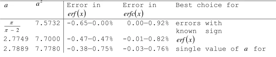
We derive a series of values for a by trial-and-error.

These values are given in Table 1, together with their accuracies when used in Eq. (7) to calculate ex2erfc

( )

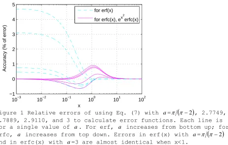
x .

The errors introduced by using Eq. (7) to estimate erf

( )

x and

( )

x

erfc are shown in Fig. 1. One can choose a value of a to evaluate the results of the error, complementary error, and scaled

[image:3.595.52.522.670.768.2]

complementary error functions easily with a calculator to within the accuracy shown.

Table 1 Values of a, errors in erf

( )

x and erfc

( )

x , and advantages of each formulation

a a2 Error in

( )

x erf

Error in

( )

x erfc

Best choice for

2 −

π

π _{7.5732 -0.65—0.00% 0.00—0.92% errors with} known sign 2.7749 7.7000 -0.47—0.47% -0.01—0.82% erf

( )

x

both erf

( )

x and erfc

( )

x 2.9110 8.4740 -0.04—3.11% -0.34—0.34% erfc

( )

x

3 9 0.00—4.70% -0.65—0.12% simple formula Examples of applications in atmospheric science

As indicated in Table 1, using a=3 results in the simplest formula:

( )

9 2 3 2 2 2 + + ≈ x x x erfc ex π

π (8)

which is never in error by more than 0.65% for complementary error and scaled complementary error functions, and which provides a neat closed solution that can be incorporated into analytical solutions for a broad range of physical and engineering problems. An example of one such problem, and the driver for the development discussed above, is the nucleation and growth of cirrus cloud

particles (Ren and MacKenzie, 2005). The approximation allowed us to describe the behaviour of cirrus clouds under all conditions, avoiding an unwieldy and unhelpful description based on asymptotic expansions to both ends when it is, in fact, the middle range that is most interesting (Kärcher and Lohmann, 2002; Ren and MacKenzie, 2005). The cirrus parameterisations are designed for

implementation in global climate models (GCMs) (Lohmann et al., 2004), where the error associated with the closed-form

approximation is small compared to uncertainty in the model output resulting from missing processes and other simplifications. There are clear advantages ⎯ in calculation speed and interpretation of results ⎯ in the use of closed-form approximations to the error and related functions within these very large GCM computer codes.

Other examples relate to normal or log-normal distributions. The size distributions of aerosols and clouds, and the parameters of turbulent processes are often log-normally distributed. Shoji and Kitaura (2006), for example, found that hourly, daily, and annual precipitation distributions were fitted well with log-normal distributions. The cumulative distribution function,D

( )

I — which indicates the probability that rainfall amount, I , will not be exceeded within period of time (hourly, daily, or annual), T — can, therefore, be given by

( )

(

)

2 2 2

1 2 1 1 ln 2 ln ln 1 2 1 2 a a ae I I erf I D m + + − − = ⎟⎟ ⎠ ⎞ ⎜⎜ ⎝ ⎛ ⎟ ⎠ ⎞ ⎜ ⎝ ⎛ − + = − πλ πλ σ λ

, (9)

where Im is the geometric mean of rainfall amount, σ is the geometric standard deviation of rainfall amounts, and

σ λ

ln 2

ln lnI − I_m

=

is a convenient measure of the position of a particular rainfall amount in the rainfall distribution. λ =1 2 when I =σI_m, λ =2 2

when I=σ2Im, and so on. You can calculate D(I) with a given λ by a

Having derived an analytical expression for the cumulative distribution function, the recurrence interval is then

( )

_{( )}

[

(

)

_{2 2 2}

]

2

1 2

1

λ

πλ

πλ a e

a a

T I D T I

R = − + +

−

= . (10)

This relatively simple expression is much easier to “read” than the equivalent retaining the error function. For instance, for I = Im, λ = 0 and so R

( )

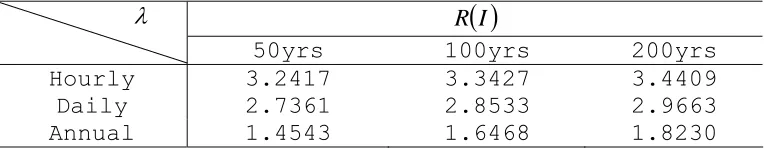
Im =2T, which confirms that there is a 50:50 chance that rainfall exceeds the geometric mean, Im. For λ =1 2,

R(σIm)≈6.3T; for λ =2 2, R(σ2Im)≈43.6T. Using Eq. (10), values of λ for the 50-, 100-, and 200-year events are given in Table 2. This time, a=2.7889 is used, as this value of a guarantees the approximation having relative errors within 0.8%. Beyond their intrinsic interest, log-normal rainfall statistics also propagate into hydrological theory — theoretical treatments of slope

stability for example (Iida, 2004) — and engineering design, where, again, avoiding the use of error functions makes model building

[image:5.595.54.436.369.444.2]

and theoretical interpretation easier (Swamee, 2002).

Table 2 Values of λ for calculating the rainfall amount at a given recurrence interval

( )

I R λ

50yrs 100yrs 200yrs

Hourly 3.2417 3.3427 3.4409

Daily 2.7361 2.8533 2.9663

Annual 1.4543 1.6468 1.8230

Conclusion

A closed-form approximation for the error, complementary error, and scaled complementary error functions with maximum relative

errors within 0.8%. Unlike other approximate solutions, this

closed-form equation gives answers within the stated accuracy for

[

∞

)

∈ 0

x . It is very useful when one wants to gain a clearer insight into the relationships between variables in a problem involving error functions.

References

Chaudhry AM, Zubair S. 1993. Analytic study of temperature

solutions due to gamma-type moving point-heat source. Int. J. Heat

Mass. Transf. 36: 1633-1637.

Cody WJ. 1990. Performance evaluation of programs for the error and complementary error functions. ACM Trans. Math. Softw. 16: 29-37.

Decker DL. 1975. Computer evaluation of the complementary error function. Am. J. Phys. 43: 833--834.

Iida, T. 2004. Theoretical research on the relationship between return period of rainfall and shallow landslides. Hydrological

Processes, 18: 739—756.

Kärcher B, Lohmann U. 2002. A parameterization of cirrus cloud formation: Homogeneous freezing including effects of aerosol size.

J. Geophys. Res. 107(D23): article 4698, doi:10.1029/2001JD001429.

Lohmann U, Kärcher B, Hendricks J. 2004. Sensitivity studies of cirrus clouds formed by heterogeneous freezing in the ECHAM GCM. J

Geophys. Res. 109(D16): D16204, doi:10.1029/2003JD004443.

Ren C, MacKenzie AR. 2005. Cirrus parameterisation and the role of ice nuclei. Q. J. R. Meteorol. Soc. 131: 1585-1605.

Shoji T, Kitaura H. 2006. Statistical and geostatistical analysis of rainfall in central Japan. Computers & Geosciences 32: 1007-1024.

Swamee PK. 2002. Near Lognormal Distribution. J. Hydro. Eng. 7: 411-444.

10−3 10−2 10−1 100 101 102 −1

0 1 2 3 4 5

x

Accuracy (% of error)

for erf(x)

for erfc(x), ex

2

[image:7.595.67.529.80.374.2]

erfc(x)