sequenceLDhot: Detecting Recombination Hotspots

SequenceLDhot: Detecting Recombination Hotspots

Paul Fearnhead

a

Department of Mathematics and Statistics, Lancaster University, Lancaster LA1 4YF, UK

ABSTRACT

Motivation: There is much local variation in recombination rates across the human genome – with the majority of recombination occu-ring in recombination hotspots: short regions of around 2kb in length that have much higher recombination rates than neighbouring regi-ons. Knowledge of this local variation is important, for example in the design and analysis of association studies for disease genes. Popula-tion genetic data, such as that generated by the HapMap project, can be used to infer the location of these hotspots. We present a new, effi-cient and powerful method for detecting recombination hotspots from population data.

Results: We compare our method with four current methods for detecting hotspots. It is orders of magnitude quicker, and has greater power, than two related approaches. It appears to be more powerful thanHotspotFisher, though less accurate at inferring the precise positions of the hotspot. It was also more powerful thanLDhotin some situations: particularly for weaker hotspots (10–40 times the background rate) when SNP density is lower (less than 1 per kb). Availability: Program, data sets, and full details of results are available at: http://www.maths.lancs.ac.uk/∼fearnhea/Hotspot. Contact: [email protected]

1 INTRODUCTION

There is currently much interest in understanding the fine-scale variation in the recombination rate across the human genome, and detecting the presence of recombination hotspots. Primarily this is because knowledge of this variation will inform the design and analysis of association studies for complex diseases [25, 6], and also because of interest in the evolutionary forces affecting recombination hotspots [8, 17, 16].

In recent years, recombination hotspots have been found by direct observation of crossovers in sperm [7, 9, 10]. While these give accurate measurements of current local recombination rates, and position of recombination hotspots, analysis of sperm is costly and time-consuming, and has so far been restricted to a small number of genetic regions.

To learn about genome-wide variation in recombination rates and hotpots, analysis of population genetic diversity data has proven more successful [1, 14, 24, 18, 5, 16], particularly due to the large amount of SNP genotype data describing genetic variation in different human populations [23].

Here we describe a new method for detecting recombination hotspots from population genetic data. This method uses the appro-ximate marginal likelihood method of [3] and is closely related to the methods described in [4] and [5]. The approach scans through a chromosomal region of interest, and considers fitting a recombi-nation hotspot at a set of possible locations (from a pre-specified

∗_{to whom correspondence should be addressed}

grid). For each possible hotspot location, a likelihood ratio statistic is calculated for the test of whether a hotspot is present. The set of likelihood ratio statistic values can be then be used to visually show the evidence for a recombination hotspot at different positions along the chromosome and to flag up likely locations for hotspots (see Section 2.3 for more details).

Whilst similar, this approach differs from those of [4] and [5]. For both these approachs the chromosomal region was split up into a series of sub-regions (defined to each contain a specified number of consecutive SNPs), and then the likelihood curve for the recombina-tion rate was calculated for each sub-region under the assumprecombina-tion of a constant recombination rate within that sub-region. (The methods described in [4] and [5] differ in how they combine the informa-tion from these separate sub-regions into evidence for hotspots at different locations.)

The advantage of the new approach described here is firstly com-putational, with CPU times being reduced by over an order of magnitude (see Section 4.1). This is because the Monte Carlo effort for calculating the likelihood ratio statistic for a hotspot at each possible position can be curtailed when it becomes obvious that eit-her teit-here is little or teit-here is overwhelming evidence for a hotspot (see Section 2.4). Secondly, the method allows for a more accurate estimate of the background recombination rate through using the PACL method of [12] (see [20] and discussion in [5]) and allows for this background rate to vary across large chromosomal regions. Finally the new approach can more accurately be applied to regions of data where the SNP density is low. For such regions, the ear-lier approaches would estimate a constant recombination rate over potentially large sub-regions, and any signal from a hotspot within that sub-region would be weakened due to the averaging of a small hotspot with larger non-hotspot (background) regions. This is avoi-ded within the new method by always fitting an appropriate hotspot model, consisting of a small hotspot region flanked by a background region.

We have compared our new method for detecting hotspots with the earlier methods of [4] and [5], as well as theHotspotFisher

program of [11] and theLDhotprogram of [14, 16].

2 METHOD

2.1 Overview of Method

Our approach is to consider a grid of possible hotspot positions, and to eva-luate the evidence for the presence of the hotspot at each of these positions. To define the grid, we specify a hotspot width,w, and a spacing,l(see Section 2.2). Assume theLSNPs are at ordered positionsx1, . . . , xL, and

without loss of generality relabel positions so thatx1 = 1. LetN be the largest integer such thatN×l+w < xL. Then our algorithm consists of

the following loop: Fori= 0, . . . , N:

(i) Consider a hotspot from positioni×ltoi×l+w. Denoteρto be the recombination rate within the hotspot andρ(bi) to be the background

recombination rate close to this hotspot.

(ii) ChooseSSNPs close to this hotspot, and summarise the data by the sequences defined solely by the alleles at theseSSNPs.

(iii) Use the Approximate Marginal Likelihood method of [3] to estimate LRithe likelihood-ratio statistic forρ > ρ(

i)

b againstρ= ρ

(i)

b , for

the data chosen in (ii).

The output of the method is a set of likelihood ratio statistics{LRi}Ni₌₀

for the presence of a hotspot of widthwstarting at positions0, l, . . . , N×l. These likelihood ratio statistics are estimated based on an Importance Samp-ling approach [2, 3]. They are estimated under a standard neutral coalescent model, though the likelihood for such a model has been shown to be robust for inference of relative recombination rates [20].

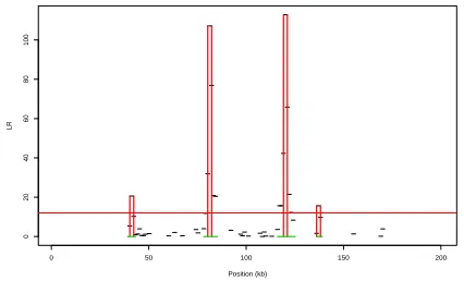
Whilst this is a non-regular inference problem, simulation studies [3, 4] suggest that the null distribution of the likelihood ratio statistic is approxi-mately an equal mixture of a point mass at 0, and a chi-squared distribution with one degrees of freedom. A plot of the likelihood ratio statistic against hotspot position (see for example Figure 1) can give a picture of the evi-dence for the presence of a hotspot against position across the chromosomal region. Details of how we use this output to give predictions for the position of hotspots is given in Section 2.3.

2.2 Details of Method

The method requires specifying a number of parameters. We describe here the default choices of our method, which are suitable for analysing human population genetic data and are the values we used for the results shown in this paper. Firstly we chose the hotspot widthw = 2000and spacing l = 1000. The width is based on evidence that hotspots are of the order of 1-2kb [7], and the spacing is based on a trade-off between computational cost and accuracy. In calculating the Likelihood ratio statistic in step (iii) we allow for a range for the hotspot recombination rate, and these where chosen to be between 10 and 100 times the background rate.

The choice of the number of SNPs,S, in step (ii) of the algorithm is again a trade-off between the information in the data summary, and the compu-tational cost and Monte Carlo error in the estimate of the likelihood ratio statistic. We choseS = 7, which appears to give a noticeable improve-ment overS= 6, while increasingSfurther did not appear to substantially improve performance.

The algorithm for choosing which SNPs to keep in step (ii) is based upon the intuition that the most informative set of SNPs will have larger minor allele frequency and be equally spaced in or close to the putative hotspot.

2.3 Summarising Output

Given the likelihood ratio statistic for one putative hotspot positionLRi,

the simplest approach is to predict the presence of a hotspot ifLRi > c

for some cutoffc. The approximate null distribution of the likelihood ratio statistic can be used to specify a suitable value forc. Values ofc= 10and c= 12would produce a false-positive approximately once every 1200 and 3700 independent tests respectively (and are what we choose for the results in this paper). Given a hotspot spacing of1kb, and making the conserva-tive approximation that tests for hotspot positions are independent, then this

0 50 100 150 200

0

20

40

60

80

100

Position (kb)

LR

Fig. 1. Example output fromsequenceLDhot. The raw output is the Likelihood Ratio values for each putative hotspot (shown by black horizontal lines if non-zero). These are converted into extended hotspot regions (deno-ted by green horizonal lines), for each such region we infer a single hotspot (position given by red vertical lines – height of lines gives the evidence for that hotspot). These results are for a cutoff ofc= 12(red horizontal line).

would suggest a false-positive rate of less than 1 per 1.2Mb and 1 per 3.7Mb respectively.

However this simple approach is likely to predict a number of hotspot positions for each true hotspot, as each real hotspot will overlap a number of the putative hotspot positions within our grid. Furthermore even a hotspot near, but not overlapping, the putative hotspot may produce some evidence of a hotspot, as its presence will reduce the amount of Linkage Disequilibrium (LD) within the sub-region covered by theSSNPs chosen in step (ii) of the method. Thus the patterns generated by theSSNPs may fit a hotspot model better than a no-hotspot model, even if the hotspot is in the wrong position.

As a result we summarise the output of our method by a set of disjoint extended hotspot regions, which are defined to be contiguous regions with evidence for a hotspot. Each extended hotspot region contains at least one putative hotspot withLR > c. Extending out from this putative hotspot we then include all hotspot positions withLR >4, and all hotspot positions that overlap with a more distant hotspot position that haveLR > c. The idea is to describe in an automated way a contiguous region that contains all hotspot positions whoseLRvalue may have been affected by the presence of the putative hotspot, and thus to avoid inferring clusters of nearby hots-pots all except one of which are likely to be false positives. (More accurate methods may be possible, but this ad hoc approach appears to work well in practice.)

Within each extended hotspot region we then infer a single hotspot, whose position is chosen to be the hotspot position with the largest likelihood ratio value within that extended hotspot region.

See Figure 1 for an example of output of our method, and the definition of the extended hotspot regions and the inferred hotspots.

2.4 Implementation

To obtain haplotype data from genotype data we usedPHASEv2.1[22, 21]. To obtain estimates of the background recombination rate we used the inferred recombination rates withinPHASEv2.1obtained under the-MR

flag [12]. These estimates are based on a model which allows a different recombination rate between each pair of consecutive SNPs. To estimate the background recombination rate at a positionxwe took the median of all the recombination rates esimated within a 100kb window centered onx. (The programsequenceLDhotis able to directly input the appropriate output fromPHASEv2.1; )

hotspot. We specified a minimum,N0and maximumK×N0number of iterations. Everyk×N0iterations, fork= 1,2, . . . , K−1we checked the current estimate of the likelihood ratio statisticLRi. IfLRi < 4or

LRi >20then we stopped the Monte Carlo simulations for that putative

hotspot. The idea is to stop the simulations if there is either little or over-whelming evidence for a hotspot. The choices of cut-off value where chosen to be a factor of roughly 2 different from the cutoffs ofLRi > 10and

LRi>12considered for detecting hotspots.

This idea of curtailing the Monte Carlo simulation in step (iii) substanti-ally reduces the computation cost of the method, and was found to have no noticeable effect on the performance of the method. For the results shown here we choseN0 = 300andK= 50. The Monte Carlo method in step (iii) uses bridge sampling [15]. For each set of 300 Monte Carlo simulations we used 100 simulation from each of 3 driving values; see [2] - one being the background recombination rate and two being rates consistent with a hotspot.

3 DATA AND OTHER METHODS

We compare our method to four recent methods, these are

(i) the Likelihood Ratio method of [4];

(ii) the Penalised Likelihood of [5], code available from http://www.maths.lancs.ac.uk/∼fearnhea;

(iii) theHotspotFisherprogram of [11] which is available from http://bioinfo.au.tsinghua.edu.cn/member/∼lijun; and

(iv) theLDhotprogram of [16].

Our comparisons were based on three sets of simulated data taken from a number of recent papers. The names we use for each set of simulations, based upon the real data the simulations try to mimic, together with brief descriptions are as follows:

SeattleSNP These data sets attempt to mimic data from the SeattleSNP, and

consist of 200 independent data sets, each for a 25kb region sampled from a European and African American population; the sample sizes are 23 and 24 individual respectively, and 100 data sets contain no hotspots, and the other 100 each contain a single hotspot. These are taken from [5].

HapMap Encode These data sets consist of one hundred 200kb regions,

sampled in three populations (European, Asian and African). Each region contains a random number of hotspots (mean close to 4), and 90% of recom-bination events occur within the hotspots. Sample sizes are 90 individuals for each population. These are the HQ= 90%data sets from [11].

Human-Chimp These data sets are taken from [24] and were generated

empirically from real data. They consist of data from 3 different Encode regions (4q26, 7q21 and 7q31), in European, African and chimp populati-ons. In humans, the average background rate in the 3 regions were 0.5–0.6 cM/Mb, 0.4 cM/Mb and 0.4 cM/Mb respectively. Each data set consists of a 100kb region with a 2kb hotspot at position 49kb-51kb. A range of hots-pot sizes were considered, and we give results for hotshots-pots of the following intensities (all cM/Mb): 0.8, 4, 8, 16, 40, 80, and 160. Sample sizes were 60, 60 and 38 respectively. SNP density varied considerably: 1.8 per kb (Euro-pean), 2.5 per kb (African), and 0.6 per kb (chimp).

For further details of these data sets, see the original papers. The Seatt-leSNP and HapMap Encode simulations both used thecosiprogram of [19].

The HapMap Encode simulate data sets are available from

http://bioinfo.au.tsinghua.edu.cn/member/∼lijun, and the other data sets are available from

http://www.maths.lancs.ac.uk/∼fearnhea/Hotspot.

4 RESULTS

We now give the results of our new method, sequenceLDhot, on the three sets of simulated data sets as described in Sec-tion 3. All simulated data sets provide genotype informaSec-tion, and

Table 1. Results for SeattleSNPs simulated data.

sequenceLDhot PL [5]a

LR [4]a

Populationb

EA AA EA AA EA AA

False Positivesc

6 2 2 5 2 4

Power (%) 73 65 63 67 56 44

a: Results taken from [5].

b: Populations are European American (EA), African American (AA). c: False positives across 200 25kb data sets for each population.

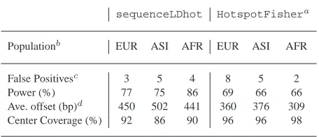
Table 2. Results for HapMap Encode simulated data.

sequenceLDhot HotspotFishera

Populationb

EUR ASI AFR EUR ASI AFR

False Positivesc

3 5 4 8 5 2

Power (%) 77 75 86 69 66 66

Ave. offset (bp)d

450 502 441 360 376 309

Center Coverage (%) 92 86 90 96 96 98

a: Results taken from [11].

b: Populations are European (EUR), Asian (ASI) and African (AFR). c: False positives across 100 200kb data sets for each population.

d: Average offset of predicted center forsequenceLDhot, and average offset of predicted start and end of hotspots forHotspotFisher.

we first inferred haplotypes and estimated background recombina-tion rates usingPHASEv2.1. For the power results we show for

sequenceLDhot, we treat a hotspot as found if it overlaps with an inferred hotspot. We count as false-positives any hotspots that do not overlap with a true hotspot. (Thus we ignore the extended hots-pot regions when calculating power and false positive rates, which makes comparisons with existing methods fair.)

4.1 SeattleSNPs

Our first comparison is with the Likelihood Ratio (LR) method of [4] and the Penalised Likelihood (PL) method of [5]. Firstly, the computation involved usingsequenceLDhotis substantially smaller than that of either of the LR or PL methods. All methods require the use ofPHASEto infer haplotypes. For an example data set sequenceLDhot took 10 minutes to analyse the resulting haplotype data; whereas both the LR and PL methods took of the order of 4 hours.

Human

Hotspot Rate cM/Mb

Power

0.8 4 8 16 40 80 160

0

0.5

1

Chimp

Hotspot Rate cM/Mb

Power

0.8 4 8 16 40 80

0

0.5

1

Fig. 2. Plot of power against Hotspot strength for Human-Chimp data: (Top)

Results for human data; (Bottom) Results for Chimp data. For each plot: (black)sequenceLDhotc= 12, (red)sequenceLDhotc= 5, (blue)

HotspotFisher; (green)LDhot. In both plots vertical bars give appro-ximate 95% confidence intervals on the estimates of power. Recombination rate for hotspot is on a log scale.

4.2 HapMap Encode

We next analysed the HapMap Encode simulated data, HotspotFisher. While each data set consists of 200kb sequenced in 90 individu-als, to speed up the implementation of our method (in particular to reduce the CPU cost ofPHASE) we subsampled just 45 individu-als, and analysed separately the first and last 110kb of sequence. We chose to split the sequence in this way so that for putative hotspots at positions close to 100kb we would still have sufficient informa-tive SNPs surrounding the hotspot that we would not suffer any loss of power. Our method then took on the order of 1–2 hours to analyse a single 200kb data set (which includes running both

PHASEandsequenceLDhot), as compared to a few minutes for

HotspotFisher.

Results are given in Table 2. When testing for hotspots we used a cut-off ofc = 12so that our method had similar false positive rates toHotspotFisher. We have a noticeable improvement in power overHotspotFisher: when averaged over three popula-tion, we have a power of 79% as compared to 67%. However, for inferred hotspots,HotspotFisheris more accurate at detecting the hotspot position.

One noticeable problem with our method is in terms of detec-ting individual hotspots when they cluster together. In these cases our method will tend to infer a large extended hotspot region, and thus a single hotspot. The power of our method increases by 8% if we include as detected all hotspots that lie fully within any exten-ded hotspot region. (The average hotspot region is around 5–6kb in length.)

4.3 Human-Chimp

Finally we analysed the human-chimp data. We ransequenceLDhot

on all data sets, andHotspotFisheron the human datasets (we had technical difficulties with runningHotspotFisheron the chimp data). We also obtained results forLDhotfrom Table S3 of [24]. These data sets only enable us to compare power (as oppo-sed to false-positive rates), as they all contain a known hotspot, but the recombination landscape in the remaining part of the region is unknown.

The results forsequenceLDhotandHotspotFishergive values for the power of the method for 7 different recombination rates of the hotspot ranging from 0.8 cM/Mb to 160 cM/Mb. (As compared to a background rate in humans of approximately 0.4 cM/Mb.) We pooled results for all three regions together, and also pooled results from both human populations.

For comparison betweensequenceLDhotandHotspotFisher

we chose a cutoff value of c = 12 as for this value the two methods had similar false positive rates for the HapMap Encode data. The resulting estimated power curves for both methods are shown by the black and blue curves in Figure 2. Again we see thatsequenceLDhotis more powerful at inferring hotspots than

HotspotFisher.

Table S3 of [24] gives power of LDhot(at a 5%significance level) for different hotspot intensities. For human hotspots, they only give power values for hotspots with intensity close to 8cM/Mb; for chimp hotspots they give power values for a range of hotspot intensities. We have plotted these values on Figure 2 (green curve). For comparison we also give power curves forsequenceLDhot

with cutoffc = 5, which gives a similar nominal significance level toLDhot. The results suggest that LDhotis more power-ful at estimating hotspots of strength close to 8cM/Mb (20 times the background rate) in the human data. For the chimp data it appears thatsequenceLDhotis more powerful for weaker hotspots (up to around 16cM/Mb; andLDhot is more powerful for inferring hotspots that are stronger than 16cM/Mb.

5 DISCUSSION

Our new method has a number of advantages over existing methods. It is substantially quicker, and appears to be more powerful than the Likelihood Ratio method of [4] and the Penalised Likelihood method of [5]. The gain in computational speed is substantial, and the new method is scalable to analysing genome-wide data. For example analysing a 200kb data set in the HapMap Encode analysis took of the order of 1–2 hours computing. So analysying a genome-wide data set would take of the order of 1000 CPU days, which is practicable as the analysis is trivially parallelisable.

Our method appears to be more powerful at detecting hotspots thanHotspotFisher, though the latter method is both quicker than ours, and can localise the position of the hotspots more accura-tely. The reason it appears more accurate at inferring the position of the hotspots is likely to be due to the finer grid it uses for putative hotspots.

A comparison withLDhotis more difficult, as this method is currently not publicly available. The comparison we did had the problem that we could only compare the power of the different methods, and not also the false positive rates. Whilst we attemp-ted to perform a comparison where the methods had similar putative false-positive rates, there was not way to check these in practice.

However, this comparison based on the published power results

LDhotsuggests thatsequenceLDhotmay be more powerful for weaker hotspots, and perhaps data with lower SNP density; whereas

would be obvious from a different choice of SNPs. This may mean it works poorly, compared to other methods, for stronger hotspots – where the occasional choice of a poor set of SNPs will limit its power slightly away from 100%. Secondly, as SNP density increases substantially (to say greater than 1 SNP per kb),sequenceLDhot

is unable to fully utilise this extra information as it always calculates the Likelihood Ratio statistics based on a fixed number of SNPs. By comparisonLDhotwill continue to be able to take account of the information in these extra SNPs regardless of how high SNP density becomes.

ACKNOWLEDGEMENT

This work was supported by EPSRC grant GR/S18786/01. The idea for this work came out of discussions with the Statistical Genetics Group, Department of Statistics, University of Oxford. I thank Simon Myers and Jun Li for making their sending me the Human-Chimp and HapMap Encode data sets respectively.

REFERENCES

[1]D C Crawford, T Bhangale, N Li, G Hellenthal, M J Rieder, D A Nickerson, and Matthew Stephens. Evidence for substantial fine-scale variation in recombination rates across the human genome. Nature Genetics, 36:700–706, 2004.

[2]P Fearnhead and P Donnelly. Estimating recombination rates from population genetic data. Genetics, 159:1299–1318, 2001.

[3]P Fearnhead and P Donnelly. Approximate likelihood methods for estimating local recombination rates (with discussion). JRSS, series B, 64:657–680, 2002. [4]P Fearnhead, R M Harding, J A Schneider, S Myers, and P Donnelly.

Applica-tion of coalescent methods to reveal fine-scale rate variaApplica-tion and recombinaApplica-tion hotspots. Genetics, 167:2067–2081, 2004.

[5]P Fearnhead and N G C Smith. A novel method with improved power to detect recombination hotspots f rom polymorphism data reveals multiple hotspots in human genes. American Journal of Human Genetics, 77:781–794, 2005. [6]J N Hirschhorn and M J Daly. Genome-wide association studies for complex

diseases and complex traits. Nature Reviews Genetics, 6:95–108, 2005. [7]A J Jeffreys, L Kauppi, and R Neumann. Intensely punctate meiotic recombination

in the class II region of the Major Histocompatibility Complex. Nature Genetics, 29:217–222, 2001.

[8]A J Jeffreys and R Neumann. Reciprocal crossover asymmetry and meiotic drive in a human recombination hotspot. Nature Genetics, 31:267–271, 2002. [9]A J Jeffreys, R Neumann, M Panayi, S Myers, and P Donnelly. Human

recombina-tion hotspots hidden within regions of strong marker associarecombina-tion. Nature Genetics,

37:601–606, 2005.

[10]L Kauppi, M P Stumpf, and A J Jeffreys. Localized breakdown in linkage dise-quilibrium does not always predict sperm crossover hot spots in the human MHC class II region. Genomics, 86:13–24, 2005.

[11]J Li, M Q Zhang, and X Zhang. A new method for detecting human recombi-nation hotspots and its applications to the HapMap ENCODE data. To appear in

American Journal of Human Genetics, 79:628–639, 2006.

[12]N Li and M Stephens. Modelling LD, and identifying recombination hotspots from SNP data. Genetics, 165:2213–2233, 2003.

[13]G A T McVean, P Awadalla, and P Fearnhead. A coalescent method for detecting recombination from gene sequences. Genetics, 160:1231–1241, 2002. [14]G A T McVean, S R Myers, S Hunt, P Deloukas, D R Bentley, and P Donnelly.

The fine-scale structure of recombination rate variation in the human genome.

Science, 304:581–584, 2004.

[15]X Meng and W H Wong. Simulating ratios of normalizing constants via a simple identity: a theoretical exploration. Statistica Sinica, 6:831–860, 1996. [16]S Myers, L Bottolo, C Freeman, G A T McVean, and P Donnelly. A fine-scale

map of recombination rates and hotspots across the human genome. Science, 310:321–324, 2005.

[17]M Pineda-Krch and R J Redfield. Persistence and loss of meiotic recombination hotspots. Genetics, 169:2319–2333, 2005.

[18]S E Ptak, D A Hinds, K Koehler, B Nickel, N Patil, D G Ballinger, M Przeworski, K A Frazer, and S Paabo. Fine-scale recombination patterns differ between chimpanzees and humans. Nature Genetics, 37:429–434, 2005.

[19]S F Schaffner, C Foo, S Gabriel, D Reich, M J Daly, and D Altshuler. Calibrating a coalescent simulation of human genome sequence variation. Genome Research, 15:1576–1583, 2005.

[20]N G C Smith and P Fearnhead. A comparison of three estimators of the population-scaled recombination rate: accuracy and robustness. Genetics,

171:2051–62, 2005.

[21]M Stephens and P Donnelly. A comparison of Bayesian methods for haplo-type reconstruction from population genohaplo-type data. American Journal of Human

Genetics, 73:1162–1169, 2003.

[22]M Stephens, N J Smith, and P Donnelly. A new statistical method for haplo-type reconstruction from population data. American Journal of Human Genetics, 68:978–989, 2001.

[23]The International HapMap Consortium. A haplotype map of the human genome.

Nature, 437:1299–1320, 2005.

[24]W Winckler, S R Myers, D J Richter, R C Onofrio, G J McDonald, R E Bontrop, G A T McVean, S B Gabriel, D Reich, P Donnelly, and D Altshuler. Comparison of fine-scale recombination rates in humans and chimpanzees. Science, 308:107– 111, 2005.