Foreign Reserve Adequacy in Sub Saharan Africa

Munich Personal RePEc Archive

Foreign Reserve Adequacy in

Sub-Saharan Africa.

Drummond, Paulo and Dhasmana, Anubha

International Monetary Fund

1 June 2008

Online at

https://mpra.ub.uni-muenchen.de/9729/

_{Foreign Reserve Adequacy in}

Sub-

_{Saharan Africa}

© 2008 International Monetary Fund WP/08/150

IMF Working Paper

African Department

Foreign Reserve Adequacy in Sub-Saharan Africa

Prepared by Paulo Drummond and Anubha Dhasmana

Authorized for distribution by Andrew Berg

June ₂₀₀₈

Abstract

This Working Paper should not be reported as representing the views of the IMF. The views expressed in this Working Paper are those of the author(s) and do not necessarily represent those of the IMF or IMF policy. Working Papers describe research in progress by the author(s) and are published to elicit comments and to further debate.

This paper looks at the question of adequacy of reserves in sub-Saharan African countries in light of the shocks faced by these countries. Literature on optimal reserves so far has not paid attention to the particular shocks facing low-income countries. We use a two-good endowment economy model facing terms of trade and aid shocks to derive the optimal level of reserves by comparing the cost of holding reserves with their benefits as an insurance against a shock. We find that the optimal level of reserves depends upon the size of these shocks, their probability, and the output cost associated with them,.

16B

JEL Classification Numbers: F32

Keywords: Foreign Exchange Reserves, Balance of Payments Crises, Terms of Trade and Aid Shocks

2

Contents Page

I. Introduction ...3

II. Foreign Reserves in sub-Saharan Africa...4

III. Shocks Facing Sub-Saharan Africa ...7

IV. Small Open Economy with Two Goods ...13

V. Simulation Results ...18

VI. Conclusion ...29

Tables 1. Comparisons of International Reserves Across Regions, 1995–07 ...5

A1. Benchmark Parameters ...33

A2. Simulation Parameters for Countries ...34

Figures 1. Reserves in Months of Imports ...4

3. Reserves to Short-Term Debt <2, 2007 ...7

4. Frequency Distributions of Key Parameters ...8

5. Frequency Distributions of Key Parameters ...9

6. Response of Key Macro Economic Variables to a Large TOT Schock ...11

7. Response of Key Macroeconomic Variables to a Large Aid Shock...12

8. Optimal Reserve Behavior – Jeanne-Ranciere v.s. Two-Good ...20

9. Path of Consumption—Ranciere vs. Two-Good Model...21

10. Optimal Reserve Behavior—Two Good Model with both TOT and Aid Shock [I] ...22

11. Optimal Reserve Behavior—Two Good Model with both TOT and Aid Shock [II] ...23

12. Actual Level of Reserves to GDP ratio for SSA countries...24

13. Sensitivity of Optimal Reserves to Key Parameters ...25

14. Sensitivity of Optimal Reserves to Key Parameters ...26

15. Reserve Adequacy for African Countries Using Two-Good Model /1 ...28

16. Country Specific Application—Illustrative Examples. ...29

I. INTRODUCTION

Policy makers in sub-Saharan Africa (SSA), as elsewhere, often need to find an operational way to assess reserve adequacy.Assessing adequacy needs to be viewed in the broader context of macroeconomic policies.A specific level of reserves may be adequate when alternative sources of financing exist or adjustment can be quickly attained. The same level of reserves, however, may not be adequate if there are no alternative sources of financing, no exchange rate instrument, and/or there is a reluctance or inability to correct a current account deficit. In addition, a large number of economic fundamentals, besides international reserves, can amplify the impact of adverse shocks and render a country crisis-prone in the event of a shock. These include risky short-term financing structures; stock imbalances due to maturity, currency, and interest rate mismatches; and high leverages in public and private sector balance sheets.

Recent studies have attempted to assess reserve adequacy by weighing the consumption smoothing benefits of holding reserves against their cost (Aizenman and Lee, 2005, Garcia and Soto, 2004, and Jeanne and Ranciere, 2006). Jeanne and Ranciere (2006) consider a small open economy with a single good consumed domestically and abroad. The economy is vulnerable to sudden stops in capital flows from abroad. Reserves allow the country to smooth domestic absorption in response to sudden stops, but yield a lower return than the interest. They come up with a closed form, analytical solution for the optimal level of reserve holdings under the above mentioned assumptions and apply it to industrial and emerging market countries. They find that under plausible calibrations the model can explain reserves of the magnitude observed in many industrial and emerging countries.

SSA countries, however, are routinely faced with substantially different shocks than

industrial and emerging market economies.These shocks include abrupt changes in the terms of trade and aid flows, which can contribute to higher volatility in aggregate output and, in extreme cases, to economic crisis. Recent reserve models of consumption smoothing do not tend to take into account exogenous shocks such as changes in terms of trade and aid flows that affect most developing countries.

4

The country simulations considered here take into account various aspects of vulnerability. Standard indicators consider financing needs (reserves/imports) and elements of balance sheet vulnerabilities (reserves/money and reserves/short-term external debt). Some of the LIC-specific indicators take into account many of the factors, notably the cost and risk of shocks and the interest cost of financing reserve holdings. The use of a small open economy two-goods model allows us to simulate the optimal level of reserves across a broad spectrum of shocks and output costs, but the “optimal level” of reserves is sensitive to the choice of key parameters such as the risk aversion, the term premium and the probability of shocks, and results in the paper are illustrative of model simulations for a given set of parameters. However, they leave many key considerations out. Inevitably, then, their application requires judgment.

The paper is organized as follows. Section II provides some background on the currently used measures of foreign reserve adequacy in Sub-Saharan African countries. Section III focuses on the specific shocks faced by SSA countries and their impact on some key macroeconomic variables. Section IV presents the basic model used for simulations that takes in to account these shocks. Simulation results from the model are presented in Section V. Section VI presents concluding remarks.

II. FOREIGN RESERVES IN SUB-SAHARAN AFRICA

A. The State of Play

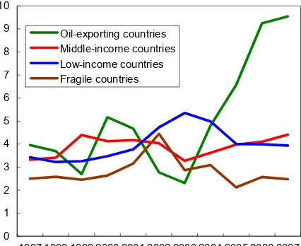
Foreign reserves for all of SSA are reached an all time high of US$127 billion in 2007. Over the past 10 years fast reserve accumulation by oil exporters and steady accumulation by South Africa are notable. This reflects low initial reserve holdings, increasing openness of SSA economies, and a policy choice to build precautionary levels to insure against balance of payment risks. Other SSA countries have kept reserves roughly stable as a share of imports (see Figure 1).

Figure 1. Reserves in Months of Imports1

0 1 2 3 4 5 6 7 8 9 10

1997 1998 1999 2000 2001 2002 2003 2004 2005 2006 2007 Oil-exporting countries

Traditional measuressuggest reserve levels vary greatly across countries and country groupings (See Figures 2 and 3).

• Current account-based measures—gross official reserves in months of imports—are particularly useful for SSA countries, as an indication of how rapidly countries would need to adjust to shocks. At end-2007, reserves covered 5.8 months of imports, up from 3.7 months in 1997-2002. This reflects a wide range across countries, though, with above average cover in oil exporting countries and below average cover in fragile countries.

• Since some of the countries in the region are also subject to potential capital outflows, capital account-based measures of reserve adequacy are important too. The ratio of reserves to short term debt, especially relevant for countries that face risks related to short-term external financing, was less than 1 for only a handful of countries.

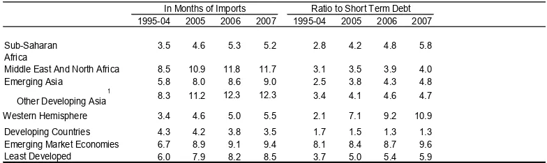
Reserve levels of other regions offer yardsticks for comparison.Reserve levels for the SSA as a whole are lower than those for the Middle East and North Africa where reserves have served as a store of value in resource rich countries, but higher than those of developing countries in general (Table 1). But with structural changes affecting balance of payments flows and the diverse macroeconomic settings and vulnerabilities of different countries, the experience of other regions provide only limited guidance for SSA countries about the adequate level of reserves in future.1 _{Also, many countries may accumulate reserves as a}

side- effect of monetary and exchange rate policies, such as efforts to stem real exchange rate appreciation. In this case, the observed level of reserves is no benchmark for adequacy.

1995-04 2005 2006 2007 1995-04 2005 2006 2007 Sub-Saharan

Africa

3.5 4.6 5.3 5.2 2.8 4.2 4.8 5.8 Middle East And North Africa 8.5 10.9 11.8 11.7 3.1 3.5 3.9 4.0 Emerging Asia 5.8 8.0 8.6 9.0 2.5 3.8 4.3 4.8

Other Developing Asia

1

8.3 11.2 12.3 12.3 3.4 4.1 4.6 4.7 Western Hemisphere 3.4 4.6 5.0 5.5 2.1 7.1 9.2 10.9 Developing Countries 4.3 4.2 3.8 3.5 1.7 1.5 1.3 1.3 Emerging Market Economies 6.7 8.9 9.1 9.4 8.1 8.4 8.7 9.6 Least Developed

Countries

6.0 7.9 8.2 8.5 3.7 5.0 5.4 5.9 Source: IMF, World Economic Outlook.

1 _{Excluding China & India.}

In Months of Imports Ratio to Short Term Debt

Table 1. Comparisons of International Reserves Across Regions, 1995-07

1

6

Reserves

in Months of Impor

ts

1

0 2 4 6 8 10 12 14

Congo, D. R. Liberia Seychelles Eritrea Zimbabwe Guinea Ethiopia Malawi Ghana Madagascar Namibia Zambia Burundi South Africa Mauritius Swaziland Cape Verde Kenya Gambia WAEMU Mozambique STP Sierra Leone Tanzania CEMAC Angola Lesotho Rwanda Uganda Comoros Nigeria C ountr y / Cou n tr y Gr oups

Reserves in Months of Imports (2007)

Reser ves as Per c entage o f M2

0 20 40 60 80

10 0 12 0 14 0 16 0 Eritrea Seychelles Mauritius South Africa Ethiopia Congo, D. R. Liberia Guinea Namibia Cape Verde Kenya Gambia Burundi Zambia Malawi WAEMU Madagascar Sierra Leone Tanzania STP Rwanda Swaziland Comoros Angola CEMAC Uganda Nigeria Lesotho Co untr y / C oun tr y G roups

Reserves as Percentage of M2

R

e

serves as

Per

c

entage of GDP

0 5 10 15 20 25 30 35

Zimbabwe Congo, D. R. Eritrea Guinea Ethiopia Liberia Malawi Seychelles Zambia Namibia South Africa Madagascar Kenya Ghana Burundi Sierra Leone WAEMU Tanzania Rwanda Mozambique CEMAC Gambia Angola Mauritius Uganda Comoros Swaziland Cape Verde STP Nigeria Co un try / Co untry Group s

Reserves as Percentage of GDP

So ur c e : W orld E c o nomic Out lo ok 1 Impor ts of Goo d

s and S

e rv ice s F igure 2. Res e rv

es in

Sub-Saharan Af

rican Count

ries

0 0.4 0.8 1.2 1.6 2

Zimbabwe Burundi Congo, D. R. Namibia Seychelles Gambia Guinea South Africa

Country/ Country Groups

R

e

serv

es to

Sho

rt-Te

rm D

ebt

Figure 3. Reserves to Short-Term Debt <2, 20071

Source: World Economic Outlook

1

Short-Term Debt by Remaining Maturity

III. SHOCKS FACING SUB-SAHARAN AFRICA

Countries in SSA face substantially different shocks compared to industrial and emerging market countries.The main shocks facing low income countries in Africa are: a sharp change in their terms of trade due to exogenous movements in the prices of key exports/imports and a change in the net aid flows (defined as Net Official Development Assistance Grants less Food and Technical assistance) received by them.

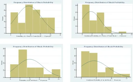
For the purposes of our analysis we define shocks in terms of annual percentage changes in terms of trade or aid flows facing a country. To further capture the idea of `large changes’ we define a terms of trade shock as an year on year decline in the terms of trade index larger than 10 percent in absolute terms. Similarly, an aid shock is defined as a decline in the net aid inflow of 50 percent or more in absolute terms. These thresholds are based on the probability distribution of the two shocks so that such events happen 20-25 percent of the time for an average SSA country2 _{(Figures 4 and 5)}

Eighty percent of the SSA countries face a 10 percent or larger negative terms of trade shock at least 5 percent of the time or more while 80 percent of these countries face a 50 percent or larger decline in aid flow at least 5 percent of the time or more. The average size of a terms of trade shock in SSA countries is 21 percent while the average size of aid shock is 181 percent (roughly 4-5 percent of GDP). Average probability of a terms of trade shock as defined above, in SSA countries, is about 20 percent and that of an aid shock is 10 percent.

2

8

Figure 4. Frequency Distributions of Key Parameters

0

5

10

15

20

25

Pe

rc

en

t

0 5 10 15 20 25

Probability of a Terms of Trade Shock < - 10 percent Frequency Distribution of Shock Probability

0

10

20

30

40

Pe

rc

en

t

0 5 10 15 20 25

Conditional Probability of a Terms of Trade Shock < - 10 percent Frequency Distribution of Shock Probability

0

10

20

30

40

P

er

cen

t

0 5 10 15 20 25

Probability of an Aid Shock < - 50 percent Frequency Distribution of Shock Probability

0

10

20

30

40

Pe

rc

en

t

0 5 10 15

Conditional Probability of an Aid Shock < - 50 percent Frequency Distribution of Shock Probability

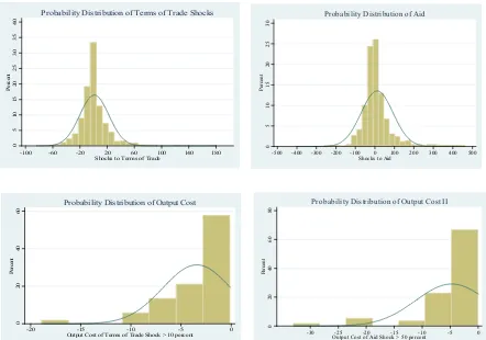
The loss in output and consumption due to such shocks can be significant, especially for countries with low levels of foreign reserves. The average loss in output, as measured by the reduction in GDP growth following a shock, associated with a 10 percent or larger terms of trade shock is 1.5 percent (based on the sample)3_{. Same is true for the output loss associated}

with an aid shock of 50 percent or more. About 40 percent of aid shocks are associated with an output cost lying between 0.5 to 4 percent and another 20 percent with an output loss between 5-6 percent. About 40 percent of the terms of trade shocks are associated with output cost of 2 percent or more.

However, the actual response of output and consumption to a shock varies significantly with the level of reserve holdings of a country. Countries with a high level of reserves to GDP ratio (those in the top 25th percentile) showed very little effect of a terms of trade or aid shock on their output and consumption. On the other hand, countries with low reserves to GDP ratio (bottom 25th percentile) showed a significant decline in their output growth and an even more dramatic decline in their per capita consumption.

3

Figure 5. Frequency Distributions of Key Parameters

0

5

10

15

20

25

30

35

40

P

er

cen

t

-100 -60 -20 20 60 100 140 180

Shocks to Terms of Trade

Probability Distribution of Terms of Trade Shocks

0

5

10

15

20

25

30

P

er

cent

-500 -400 -300 -200 -100 0 100 200 300 400 500 Shocks to Aid

Probability Distribution of Aid

0

20

40

60

P

er

cent

-20 -15 -10 -5 0

Output Cost of Terms of Trade Shock > 10 percent

Probability Distribution of Output Cost

0

20

40

60

80

P

er

cent

-30 -25 -20 -15 -10 -5 0

Output Cost of Aid Shock > 50 percent

Probability Distribution of Output Cost II

Figures 6 and 7 provide some evidence on the response of absorption, output, and foreign reserves to large terms-of-trade and aid shocks over the period 1980-2006. We classify countries as ‘Low-Reserve’ (LR henceforth) or ‘High Reserve’ (HR henceforth) based on their average reserve-to-GDP ratio during 2000-06. Of the 44 SSA countries, eleven

countries whose average reserve-to-GDP ratio was in the bottom 25th percentile were called LR countries. Overall average reserve to GDP ratio for this group during this period was 4.2 percent.

Countries in the HR group had an average reserve to GDP ratio higher than 16 percent during 2000-06 and the overall average for the period was about 28 percent ( 7 times more than that for LR countries).

We then identify the ‘shocks’, as defined in the beginning, for these countries over a period of 27 years (1980-2006).4 _{Next we look at the behavior of GDP growth, domestic absorption}

(defined as domestic consumption plus gross capital investment per capita.) and foreign

4

10

reserves over a five-year `event’ window centered around the shock occurring at time zero. This is done for aid and terms of trade shocks separately. Events that occur inside the five-year window of the previous shock episode are excluded. The solid lines in the panels are the path of these variable in response to a terms of trade / aid shock while the broken lines give the one standard error band.

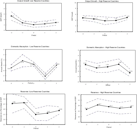
Looking at the top column in Figure 6 we can see that LR countries face a more significant decline in their GDP growth due to a terms of trade shock as compared to the HR countries. The difference is even more striking when it comes to the response of per capita absorption. For LR countries growth in per capita absorption declines significantly (it is in fact negative for one year after the shock) and does not return to the pre-shock level even after 2 years. On the other hand there is no significant change in domestic absorption for HR countries in response to a large TOT shock. It appears that countries with a higher level of reserves are better able to cushion the effect of a shock by utilizing their reserves in the event of a shock. Last column of the same panel, which plots the movement in reserves as a percentage of GDP around the shock, gives some evidence to support this view. Both LR and HR countries accumulate reserves during ‘normal’ times (i.e. before the shock) and draw down these reserves during a TOT shock (as shown by a fall in reserve level at time zero). However, while this fall in reserves amounts to about 1 percent of GDP for LR countries, for HR countries this reduction amounts to roughly 1.6 percent of their GDP. Looking at the

cumulative reduction in reserves over the two years starting with the shock, the reduction in reserves for LR countries is only 0.98 percent while it is about 3 percent for HR countries.

Clearly it is more difficult for LR countries to cushion their output and consumption in the event of a shock. In fact, unlike HR countries which continue to draw down their reserves for another year after the shock the LR countries are seen to start building their reserves

immediately after the shock. One potential reason for this may be that with already low level of reserves, LR countries can not draw down on these any further without inducing panic in the domestic and international financial markets and thereby increasing the risk of an economic crisis.

Looking at the case of a large aid `shock’ we find similar results. Output and domestic absorption are affected more in case of LR countries except that in this case the decline in domestic absorption occurs one year after the shock. This may reflect the difference between the timing of disbursement and utilization of aid proceeds. Also, as was the case with a terms of trade shock, absorption is affected more severely than output indicating the role of

consumption smoothing. To the best of our knowledge the empirical evidence provided above has not been recorded anywhere else and exploring the relationship between the level of reserve holdings and response of key macro-economic variables would be a fruitful area of future research.

cases, to economic crisis. Assessing the adequacy of reserves, thus, requires understanding the role of reserves in smoothing domestic absorption in response to external shocks, the object of the next section.

Figure 6. Response of Key Macro Economic Variables to a Large TOT Shock

Output Growth Low Reserve Countries

5.31 2.91 2.79 2.10 2.41 0 2 4 6 8 10

-2 -1 0 1 2

Period

GDP Gr

o

w

th

Output Growth - High Reserve Countries

4.77 4.39 3.76 3.88 4.89 0 2 4 6 8 10

-2 -1 0 1 2

Period

GDP Gr

owth

Domestic Absorption - Low Reserve Countries

2.03 -2.2 2.37 3.71 1.01 -4 -2 0 2 4 6 8

-2 -1 Period0 1 2

An nu al Growt h (% )

Domestic Absorption - High Reserve Countries

-0.54 2.69 1.70 1.29 2.54 -4 -2 0 2 4 6 8

-2 -1 0 1 2

Period An nu al G row th( % )

Reserves -Low Reserves Countries

4.65 3.88 3.62 3.49 4.56 2.5 3.0 3.5 4.0 4.5 5.0 5.5

-2 -1 0 1 2

Period R e s e rv es as a P e rc en tag e o f G D P

Reserves - High Reserves Countries

28.7 27.7 29.1 30.7 26.7 15 20 25 30 35 40

-2 -1 0 1 2

Period R e s e rv es a s P e rc ent ag e o f G D P

12

Figure 7. Response of Key Macroeconomic Variables to a Large Aid Shock

Output Growth Low Reserves

9 10 3.4 1.7 2.6 4.7 6.6 0 1 2 3 4 5 6 7 8

-2 -1 0 1 2

Period

GDP Gr

owth

Output Growth - High Reserves

9 10 4.8 4.2 4.9 5.1 4.3 0 1 2 3 4 5 6 7 8

-2 -1 0 1 2

Period GD P Gro w th

Consumption Growth - Low Reserve

-6.4 4.1 6.8 5.7 1.3 -15 -10 -5 0 5 10 15

-2 -1 0 1 2

Period Co nsumpt ion G row th

Consumption growth - High Reserves

2.8 -2.0 2.7 4.1 2.5 -15 -10 -5 0 5 10 15

-2 -1 0 1 2

Period C onsumpt ion G rowt h

Reserve Behavior - Low Reserves

5.3 7.9 6.8 5.1 4.2 0 2 4 6 8 10 12 14

-2 -1 0 1 2

Period Res erv es a s % of G D P

Reserve Behavior-High Reserve Countries

26.3 28.1 27.5 26.2 26.6 15 20 25 30 35 40

-2 -1 _Period0 1 2

Re ser v es as % of G D P

IV. SMALL OPEN ECONOMY WITH TWO GOODS

Consider a Small Open Economy (SOE) with two goods—one tradable and another non-tradable. The economy follows a deterministic path for the output of two goods, disturbed only by exogenous shocks to the terms of trade. Besides it gets a unilateral transfer of tradable good from abroad called “Aid” which grows at the same rate as output and is stochastic in nature. To elaborate further, a shock to the terms of trade is defined as a fall of ten percent or more in the terms of trade from the ‘normal’ level, which is set equal to one. Aid shock is also defined as an unforeseen drop in aid flows of five percent or more. In periods with no shocks, terms of trade and aid flow remain at their normal level. Probabilities of the two shocks are exogenously given as π_TOT andπ_Aid

T T

t t t t

C T Y Z A

and the two shocks are independent of each other. When either of these shocks occur, two things happen – one, output growth falls below its ‘normal level’ and second, in the case of external private borrowing, there is not roll over of short-term private external debt. Thus, aid and T.O.T shocks are always accompanied by a ‘Sudden-Stop’ in capital. The domestic economy is composed of the private sector and the government. We present two cases: with and without private external borrowing.

A. No External Private Borrowing

The representative private consumer is subject to the following budget constraints:

= × + +

N N

t t

C =Y

T t

C C_tN

T t

Y N

t

Y

t

A broad

(1.1)

(1.2)

Here is the consumption of tradable good in period t and is the consumption of non-tradable good. and are the period t output of tradable and non-tradable goods respectively. T is the terms of trade. is the unilateral transfer of tradable good from a which is given directly to the representative private consumer and consumed in the same period. Zt is t transfer of tradable good by the government. In every period the

consumption of non-tradable good is equal to its output (for simplicity we assume that the non-tradable good can not be saved). The consumption of tradable good on the other hand equals the sum of the output of tradable good, government transfer of tradable good and aid flow from abroad every period.

he

Combining equations 1.1 and 1.2 we get the over budget constraint for the consumer,

(1.3)

T N N T N N

t t t t t t t t

14

N t

P is the endogenously determined price of non-tradable good. Output of tradable as well as non-tradable good grows at the same constant rate `g’ until a terms of trade or aid shock occurs. The shock is associated with a fall in output by a fraction γ . After the shock the output goes back to its long-run path.

Denoting the periods before, during and after the shock with the sub-scripts b, d and a we can write the following equations summarizing our assumptions,

(1.4)

, (1 ) 0 , (1, )(1 ) 0 , (1, )(1 ) 0

T t T T t T T t T

t b t d t a

Y = + g Y Y = −γ + g Y Y = −γ + g Y

, (1 ) 0 , (1, )(1 ) 0 , (1, )(1 ) 0

N t N N t N N t N

t b t d t a

Y = +g Y Y = −γ +g Y Y = −γ +g Y

(

)

(

(

)(

)

, 1 0, , 1 1 0, , 1 1 0

t

t b t d Aid a Aid

(1.5)

)(

)

t t

t

A = +g A A = −γ +g A A = −γ +g A (1.6)

The government can issue a long-term security that does not have to be repaid during the shock (there is just one long-term security though there are two shocks). The long-term security issued by the government is a bond that yields one unit of good in every period until the shock occurs. The security stops yielding any income after the shock.

The pre-shock price of the security is equal to the present discounted value of the one unit of good it pays in the next period plus the expected market value of the security,

(

)

1

1 1 s

P= + −π .P

1+ +r δ ⎡⎣ ⎤⎦

Where πs =πTOT +πAid −πTOT ×πAid

r

is the probability of a shock (to aid, terms of trade or both) occurring in any period, is the short term interest rate (equal to the discount rate of the representative consumer) and δis the term premium. This implies,

1

P

r δ π_s

=

+ +

t t

(1.7)

Equation 1.7 uses the fact that the price of the long-term security is constant before the sudden stop and falls to zero when sudden stop occurs.

The government issues the long-term security to finance a stock of reserves,

R =PN (1.8)

Where is the number of securities issued by the government in period t. Government’s budget constraint is given by:

t

(

) (

)

1 1 1 1

t t t t t t

Z +R +N₋ =P N −N₋ + +r R₋ (1.9)

ation 1.8 can be used to substitute out Nt and Nt 1

Equ ₋ from equation 1.9 to get the following

expression,

(

)

1 1

1 b

t t s t

Z r R R

P − δ π −

⎛ ⎞

= −_⎜ − _⎟ = − +

⎝ ⎠ (1.10)

Negative transfer implies that the government taxes the representative consumer in order to

and when ent on

pay for the cost of carrying the reserves, which is proportional to the term premium plus the probability of a shock.

If the shock occurs, the government transfers the reserves (net of last paym the long-term security) to help the representative consumer,

(

)

d

t s t

Z = − −δ π R₋ (1.11)

fter the shock the governments become inactive and R N_t, _t and Z_t are all equal to zero. A

Using equations 1.10 and 1.11 we can get the expressions for tradable consumption before and after the shock,

(

)

, , 1

T T

t b t b s t t

C =T Y× − δ π+ R₋ +A (1.12)

(

)

, (1 ) , 1 1

T T

t TOT TOT t d s t t

C = −γ × ×T Y + − −δ π R₋ +A (1.13)

(

)

(

)

t Aid Aid t

CT_, T _,T 1 ₁ γ ×A

t d s t

Y δ π R₋

= × + − − + −

(

)

(1.14)

(

)

(

)

, , 1 1

t TOT Aid = − π R + −γAid t

, ,

T T

t a t a t

C T Y A

,

1 1

T T

TOT t d s t

C γ × ×T Y + − −δ ₋

= × + (1.16)

creasing R_t−1 raises the consumption of tradable good in period t if there is a shock and ,

, ,

t b t a t a

C Y C Y (1.17)

overnment chooses R so as to maximize the welfare of the representative consumer,

(

) (

)

0 0

1 s ,

t t s

s

U E r u C

∞

− + =

In

lowers it if there is no shock. Expression for the consumption of non-tradable is as follows

N N

, , , , , ,

N N N N

t b Ct d Yt d

= = =

G

⎡ ⎤

=

∑

here the flow utility function has a constan tive risk aversion

W t rela σ,

( )

1

C u C

σ

− ₋

=

− ,

16

( ) ( )

i T N

,i t i,

C_t = C_t α C −α; i = b, TOT, Aid

i s

C

substitution between the tradable

is the commonly used Cobb-Douglas consu ptim on aggregator with constant elasticity of

α is the sh

and the non-tradable goods and are of tradable

good in total consum er is equal to the rate

of

ption. The discount rate of representative consum

interest r. This ensures that the consumer’s maximization problem is well defined in the absence of endogenous discount rate or upward sloping interest rate function. Since Rt only affects the level of consumption in the next period, government’s problem is to choose the level of Rt n each period that maximizes the level of expected utility u C

(

)

(

)

(

)

( )

(

)

(

)

(

)

Aid TOT Aid u Ct

π π π

+ − × ×

The first order condition for the problem

(

)(

)

( )

(

)

0 1 1 1

,

arg max arg max(1 ) b TOT

t t s t TOT Aid t

Aid TOT Aid

R = E _⎣⎡u C₊ ⎤_⎦ = −π ×u C₊ + π −π ×π ×u C₊

1 πTOT πAid u Ct 1

+ + × × + is,

( )

)

(

)

(

)

s s T t

TO T

TO T Aid T t

Aid

T t

u C

u C

u C

π δ π

π π

+

+

+

− +

(

⎡

(

) (

)

' ,

s Aid TO T Aid

TO T A

δ π π π π

π π ⎤ × × − ⎢ ⎥ ⎢

(

)

id

TO T Aid uT Ct+

⎥ = − − + − × × ⎢ ⎥ ⎢_{+ × ×} ⎥ ⎣ ⎦ (1.19) serves cond

on a shock. The lef arginal cost

of reserves conditional on there bein vel of reserves is chosen

ptimally, the marginal utility of hold es is equal to the marginal cost of holding

d ption in the absence of a shock by

The right-hand side of equation 1.19 is the expected marginal utility of re itional t-hand side is the probability of no shock times the expected m

g no shock. When the le ing reserv

o them.

Denoting the marginal rate of substitution between consumption in the event of a shock an

consum ptwe can write,

( )

( )

E u C

p

E₀ u_T C_t

⎡ ⎤ ⎣ ⎦ = ⎡ ⎤ ⎣ ⎦ (1.20)

1 1 1 1 s s p s δ π

δ π δ π

+

= = −

− − − − (1.21)

e Notations, Som

(

) (

)

(

) (

)

(

) (

)

( ) ( )

TOT T N

t t TOT t TOT

Aid T N

t t Aid t Aid

TOT Aid T N

t t TOT Aid t TOT Aid

b T N

t t b t b

C C C

C C C

C C C

C C C

α α α α α α α α − − − − = = = = (1.22)

( )

(

)

(

(

) (

) (

)

)

, ,

TOT T N

TOT TOT Aid Ct Ct TOT Ct TOT

σ α α

π π π − − −

⎡ _{− × ×} ⎤ ⎢ ⎥ ⎢ ⎥

(

)

(

( ) (

) (

)

)

(

)

)

0 , ,

1 1

, ,

d Aid T N

T t Aid TOT Aid t t Aid t Aid

Aid

E u C C C C

C

σ α α

α

α π π π − − −

− ⎡ ⎤ = ⎢+ − × × ⎥ ⎣ ⎦ _{⎢ ⎥} ⎢ ⎥ ⎢ ⎥ ⎣ ⎦ (1.23) And,

(

) (

)

(

TOT Aid T N

TOT Aid Ct Ct TOT Aid t TOT

σ α

π π − −

+ × ×

( )

(

)

(

( ) ( ) ( )

)

,

T N

t b

C

'

0 1 ,

b b

T t s t t b

E u C C σ C α −α (1.24)

values of parameters and shocks.

B. External Private Borrowing

allow private external borrowing. We assume that the presentative agent can engage in short-term borrowing from abroad and that the short-term external debt (which

α π − −

⎡ ⎤ = − ×

⎣ ⎦

equations 1.21, 1.22, 1.23 and 1.24 we can simulate the optimal level of reserves for different

We modify the above framework to re

is a fraction λ of tradable good output) grows at the same rate as output until a shock occurs. This debt has to be repaid in terms of tradable good even when

he there is a shock to the terms of trade or aid, with an interest rate r. There is no default. In t event of a shock the agent repays its outstanding external debt but can not engage in fresh borrowing during or after the shock (no debt roll over). This assumption is necessary for keeping the reserve management problem meaningful since without the no-debt-roll-over condition private agent will be able to smooth over its consumption by engaging in external borrowing. These assumptions can be expressed as follows,

0

(1 ) , 0

b t T d a

t t t

18

Consumption of tradable good in each period is equal to,

(

)

T T

Y L r L Z

= × + − + ₁+ +

t t t t t t

C T ₋ A

Thus, the expression for tradable good consumption before, during and after a shock is,

(

)

(

)

, , 1 1

T T

t b t b t t s

C = ×T Y + − +L r L₋ − δ π+ R_t−1+A_t (1.26)

(

)

(

)

, (1 ) , 1 1 1 1

T T

t TOT TOT t d t s t t

C = −γ × ×T Y − +r L₋ + − −δ π R₋ +A (1.27)

(

)

(

)

(

)

, , 1 1 1

T T

t d t s t

Y r L₋ δ π R

= × − + + − − ₁ 1

t Aid Aid

C T ₋ + −γ

(

)

(

)

(

)

(

)

, , 1 , 1 1 1 1 1

t TOT Aid TOT t d t s t A

CT = −γ × ×T YT − +r L₋ + − −δ π R₋ + −γ

, ,

T T

t a t a t

C T Y A

× (1.29)

= × +

g these modified expressions in equations 1.22, 1.23 and 1.24 will give us serves with short term external borrowing.

(1.30)

eplacin vel of re

s does not allow for an analytical

lution. We therefore u al reserves as a

function of output. Simu 5_.

eter values have b countries. Average size of a

terms of trade ‘shock’ ac cent while that of an aid shock

R optimal

le

V. SIMULATION RESULTS

he two-good model presented in the above paragraph T

so se numerical techniques to solve for the level of optim

lation results presented below assume external private borrowing

A. Choice of Parameters

able A.1 gives the value of key parameters used for benchmark simulations. These T

param een calibrated using data for 44 SSA

ross SSA countries was about 21 per

was 1.8 percent (4-5 percent of GDP). These were used to calibrate γTOT _and γAid_{. Sim} average probabilities of a terms of trade shock and an aid shock were used to calibrate TOT

ilarly π

and πAid _{respectively. Aid as a share of G.D.P is equal to 4 percent (equal to a age aid to} GDP ratio for the 44 SSA countries between (1975-2005). Output cost of term

aid shocks, 1

ver

s of trade and γ _and γ_{2, were calibrated based on the impulse responses discussed in section}

III. Potential output growth, g, is set to be 5 percent based on the average growth rate for Africa over last 5 years. Share of short term debt in GDP, λ, was again calibrated using country-specific data for the 44 SSA countries for 2007. Risk free short-term rate of return, r, is set at 5 percent – same as the federal funds rate during 1987-2005. Term premium, δ ,

5

which reflects the cost of holding reserves, is set at 1.5 perc nt. This is equal to the value used by Jeanne and Ranciere (2005). One can argue that the cost of holding foreign reserves is higher in low-income African countries than in emerging market countries and therefore the term premium should be slightly higher for these countries. This value is also likely to differ across countries, and if available, country specific term-premia should be used. The remaining parameters are obtained from other low-income country studies.

B. Jeanne-Ranciere and the Two-Good Model e

this sectio the

Two-ood m

oses of

In n we compare the results from Jeanne-Ranciere model with those from

ake the comparison meaningful we do not incorporate aid shocks as of yet

G odel. To m

in the Two-Good model. In fact,we assume aid flows to be equal to zero for the purp

this exercise. In effect there is just one shock which takes a different interpretation in the case of a Two-Good model and has a direct effect on the level of tradable income. Figure 8 plots the level of optimal reserves (expressed as a percentage of G.DP.) against key parameters for both the models (remaining parameters are kept constant and same across the two models). For both the models the level of optimal reserves increases with the probability and the output cost of the shock and declines with the term premium δ . Optimal level of reserves also go up with the size of terms of trade shock in case of the Two-Good model. However, for relevant ranges of the key parameters , the Two-Good model suggests a higher level optimal reserves when compared to the Ranciere model.

To understand these results we look at the key differences between the Ranciere model and

the two-goods model. Firstly, the Two-Good model allows us to take in to account the direc

ffect of a fall in the terms of trade on the ability of the developing coun

of

t try to import tradable

ut (and consumption), but reserves can only be used to cushion the

sumption and total utility is ha e

goods. This can be called as the – ‘direct income effect’ of a fall in the relative price of a country’s exports.

Second, return to an additional dollar of reserves in terms of non-shock dollar is lower in the model with two-goods. This is because a terms of trade shock affects both non-tradable an tradable goods outp

d

r words, decline in tradable goods consumption and a lower non-tradable consumption implies a lower marginal utility of tradable consumption.

Finally, the substitution of tradable consumption between shock and non-shock states is easier in the case of the two-goods model, since tradable goods only account for half the total

consumption (its impact on the overall con lf). In othe

20

While the first point implies a higher optimal level of reserves in the two-goods model, the last two points imply a lower level of optimal reserves. For the relevant range of key parameters in question the first effect dominates the last two effects and hence the optimal

f trade

1

Broken line shows the results for Jeanne-Ranciere while the solid line shows the Two-Good model.

2

Optimal Reserves are expressed as a percentage of output.

ck of average size at time zero

ls level of reserves as a share of output is higher in the model with two goods. This in turn implies that under the benchmark parameters, the fall in consumption due to a terms o shock would be smaller in the two-goods model. For the set of benchmark parameters given in Table A .1, the Two-Good Model suggests an optimal level of reserve that is greater by about 2 percent of GDP than the one suggested by the Ranciere model.

Figure 8. Optimal Reserve Behavior – Jeanne-Ranciere vs. Two-Good Model 1,2

Figure 9 below shows the path of consumption (expressed as a percentage of GDP in the year before the shock) in the event of a terms of trade sho

when optimal reserves are chosen under the two-goods model. We compare it with the path under the Ranciere model for illustrative purposes. In the one-good model consumption fal by about 4 percent whereas it falls by only 1.5 percent in the case of the two-goods model.

0.1 0.12 0.14 0.16 0.18 0. 1 2 0. 1 3 0. 1 4 0. 1 5 0. 1 6 0. 1 7 0. 1 8 0. 1 9 0. 2 0. 2 1 0. 2 2 0. 2 3 0. 2 4 0. 2 5 0. 2 6 0. 2 7 0. 2 8 0. 2 9 0. 3 0. 3 1 0. 3 2

Probability of Shock.

O pt im a l R e s er v es as S h ar e o f O ut p ut . 0.2 Two-Good Model Ranciere 0.12 0.13 0.14 0.15 0.16 0.17 0.18 0.19 0.20 0.21 0. 0 1 0. 0 2 0. 0 2 0. 0 3 0. 0 3 0. 0 4 0. 0 4 0. 0 5 0. 0 5 0. 0 6 0. 0 6 0. 0 7 0. 0 7 0. 0 8 0. 0 8 0. 0 9 Output Cost O pt im al R es er v es a s a S har e of O ut put. Two-Good Model Ranciere 0.18 0.10 0.11 0.12 0.13 0.14 0.15 0.16 0.17

0.025 0.027 0.029 0.031 0.033 0.035 0.037 0.039 0.041 0.043

Term Premium - Delta

O p tim a l R e s e rv es as a S har e of O u tput

Two Good Model Ranciere 0.12 0.13 0.14 0.15 0.16 0.17 0.18 0.19 0. 1 5 0. 1 6 0. 1 6 0. 1 7 0. 1 7 0. 1 8 0. 1 8 0. 1 9 0. 1 9 0.2 0.2 0. 2 1 0. 2 1 0. 2 2 0. 2 2 0. 2 3 0. 2 3 0. 2 4 0. 2 4 0. 2 5 0. 2 5

Size of Terms of Trade Shock

O p tim a l R e s e rv es as a S h ar e o f O u tp ut.

Clearly, for countries facing exogenous shocks such as a terms-of-trade fall, it is important to take in to account those shocks while assessing the adequacy of their reserve holdings.

Figure 9. Path of Consumption - Ranciere vs. Two-Good Model

80 85 90 95 100 105 110 115 120

-2 -1 0

Tim

Consumption as a Share of Output in t-1

1 2

e

Ranciere Two Good Model

C. Adding Aid Shocks to the Framework

In this section w ent the results for the

full model. The two shocks in the model occur independently of each other. We use this

s with the output cost associated with each shock. Along with the actual size of the shock, the output loss associated with each shock

e

f e add the aid shocks to our Two-Good model and pres

assumption to make calculations simple since there is empirical evidence to show that the two shocks are uncorrelated (Dhasmana, 2007). Figures 10 and 11 show the results from the complete model. As before, the optimal level of reserves increases with the probability and size of terms of trade and aid shock. A higher probability of shock implies a higher expected loss in the utility due to the shock and therefore a higher optimal level of reserves. Similar argument holds for the case of size of shocks. Since the loss of consumption that a country will have to face in the event of a shock is directly related to the actual size of the shock, a country which is subject to large movements in its terms of trade or aid flows, should optimally hold a larger stock of reserves.

The optimal level of reserves also increase

determines the fall in consumption and therefore, the loss in marginal utility, associated with it. Finally, increase in the term premium lowers the optimal level of reserves that th

22

premium parameterdetermines the cost of carrying reserves in terms of reduced consum before the shock. The higher the term premium, the bigger the cut in pre-shock consumpt that the country has to take in order to finance higher consumption during the shock and therefore, lower the optimal level of reserves.

ption ion

Figure 10. Optimal Reserve Behavior—Two Good Model with both TOT and Aid Shock [I]1

0.26 0.15

0.12 0.13 0.14

0.14 0.17 0.20 0.23 0.26 0.29 0.32 Probability of Terms of Trade Shocks

Op

ti

m

al

R

eserv

es.

0.06 0.10 0.14 0.18 0.22

0.05 0.11 0.17 0.23 0.29 0.35 0.41 Size of Terms of Trade Shocks.

Op

ti

m

al

Reserv

es

0.110 0.115 0.120 0.125 0.130

0.005 0.02 0.035 0.05 0.065 0.08

Output Cost of Terms of Trade Shock.

Op

timal R

eserv

es.

0.12 0.13 0.14 0.15 0.16

1.0 1.3 1.6 1.9 2.2 2.5 2.8 3.1 3.4 3.7 4.0 Term Premium Delta (%).

Op

timal Reserv

es

1

Optimal Reserves are expressed as a percentage of output.

ves given by the Two-Good model equal to 11 to 12 percent of total output. Thus, according to the Two-Good model, a typical For the benchmark parameters, the optimal level of reser

is

countries had adequate or more than adequate reserves at the end of 2007 according to our model, there were a few whose reserve levels were significantly below the benchmark optimal given by the same model. This may be a cause of concern since SSA countries are often subject to multiple shocks at the same time and holding reserves significantly belo optimum can make them even more vulnerable to the possibility of economic crisis due to exogenous shocks.

Figure 11. Optim

w the

al Reserve Behavior—Two Good Model with both TOT and Aid Shock [II]1

0.131 0.132 0.133 0.134 0.166

0.95 1.01 1.07 1.13 1.19 1.25 1.31 Size of Aid Shock

Op

ti

m

a

l Re

s

e

rv

e

s

0.115 0.120 0.125 0.130 0.135 0.140 0.145

0.005 0.015 0.025 0.035 0.045 0.055 0.065 0.075 Output Cost of Aid Shocks

Op

tima

l R

e

s

e

rves

0.150 0.154 0.158 0.162

0.04 0.07 0.10 0.13 0.16 0.19 0.22 Probability of Aid Shocks

Opt

im

a

l R

e

s

e

rv

es

.

serves are expressed as a percentage of output.

1

24

Figure 12. Actual Level of Reserves to GDP ratio for SSA countries

0 0.05 0.1 0.15 0.2 0.25 0.3 0.35 0.4

Res

erv

e

s

t

o GDP

Rat

io f

or

44 S

S

A

C

ount

(end

2007

)

0.45 0.5

ri

es

Actual Reserves end 2007 Optimal Level Two-Good Model

However, results based on average parameter values can be misleading if there is large ariation across countries. We therefore present sensitivity analysis and some country

nsitivity Analysis.

Figures 13 and 14 show t reserves to the choice of some

key parameters. As in the figure above, we plot the actual reserve to GDP ratio for SSA

f

e

k hock

e of v

specific results in the next two sections.

D. Se

he sensitivity of the level of optimal

Figure 13. Sensitivity of Optimal Reserves to Key Parameters/1

0 0.1 0.2 0.3 0.4 0.5

Re

s

e

rv

e

s

t

o

G

DP

Rat

io

.

Prob. of Shock =

0.0 0.1 0.2 0.3 0.4 0.5

Size of TOT Shock =- 0.4 Size of TOT Shock = -0.02

0.02 Prob. of Shock = 0.3

R

e

se

rv

e

s

to

G

D

P R

a

ti

o

0 0.1 0.2 0.3 0.4

0.5 0.5

Term Premium = 0.005 _{Output Loss = 0}

0 0.1 0.2 0.3

0.4 _{Output Loss = 0.15}

Re

s

e

rv

e

s

to GDP

R

a

ti

o

Term Premium = 0.05

R

e

s

e

rv

e

s

to

G

D

P

Ratio

Sources: WEO and AFR Database.

1

26

Figure 14. Sensitivity of Optimal Reserves to Key Parameters1

0 0.1 0.2 0.3 0.4 0.5

Res

e

rv

es

to GDP

Ratio.

0 0.1 0.2 0.3 0.4 0.5

Probability of Aid Shock = 0 Probability of Aid Shock = 0.2

Re

s

e

rv

es

t

o

GDP

Ra

ti

o

Output Cost of Aid Shock = 0 Output Cost of Aid Shock = 0.15

0 0.1 0.2 0.3 0.4 0.5

Size of Aid Shock = 0 Size of Aid Shock = 2

R

e

ser

v

e

s

to

GD

P

R

a

tio

Sources: WEO and AFR Database

1

The graphs above show the sensitivity of optimal reserves to the size and probability of Aid shocks and the output cost associated with them.

E. Country Specific Applications with Sensitivity Analysis

The results above show that the choice of key parameters can affect the level of reserves that would be optimal for a particular country. In this section we use some country specific parameters alongside a few common parameters to obtain country specific estimates of optimal reserves for the SSA countries. We use data from 1980-2006 to estimate the

shock events during 1980-2007 divided by the total number of years for each country whereas the share of tradable good is calculated by multiplying the share of consumption in domestic demand with the share of imports in total consumption. Term premium δ is set equal to 1.5 for all countries (same as that used for the emerging markets by Jeanne and Ranciere). Figure 15 below plots the level of actual reserves at the end of year 2007 against the optimal reserve level, as determined by our model, for SSA countries. Both, the actual and the optimal level of reserves are expressed as a ratio of GDP.

The broken blue line is the 45 degree line which identifies countries holding an actual reserve level equal to the optimal for them. Countries to the right of this blue line hold more reserves than the optimal level indicated by our model. This can be due to several reasons – an un-anticipated surge in price of oil or other major exports increasing the government revenues or domestic money supply (thereby forcing government to undertake sterilization operations) or excessive dependence on a non-renewable resource for export revenues (e.g. diamonds in Botswana) that is likely to be exhausted in foreseeable future.

Countries to the left of the 45 degree line are those carrying fewer reserves than suggested by our model. A few of these, such as Burundi and the Democratic Republic of Congo seem to have reserve levels that are way below the optimal. Deciding upon the actual reasons and remedies for inadequate reserve accumulation requires us to look at each country separately.

28

Figure 15. Reserve Adequacy for African Countries Using Two-Good Model

CPV

KEN

NGA SEN

SYC

AGO

BEN BFA

BDI CMR CAF

CHD COM COD

COG

CIV ETA

ETH

GAB

GMB

GHA GIN

GNB

MDG

MWI _MUS

MOZ NMB

NER STP

SLE SAF

SWZ TZA TGO

UGA ZMB

0 0.1 0.2 0.3 0.4

0 0.1 0.2 0.3 0.4

Observed reserves-to-GDP ratio (2007)

Op

ti

ma

l

rese

rves-to-GDP

ra

tio ba

s

e

d on

t

w

o-go

od

mo

d

el

Sources: WEO and AFR database

Figure 16 below illustrates the application of our model for assessing reserve behavior for individual countries, illustrated by a set of two countries. It plots the actual and `optimal’ level of reserves along with the ‘reserve gap’—all expressed as a percentage of GDP, for Angola and Congo, D.R.for the years 2000-07.

The reserve gap is defined as the difference between optimal level of reserves, as suggested by our model and the actual level of reserves. We use a combination of country specific and common parameters to simulate optimal level of reserves for each country over time. In particular, the probability of aid and terms of trade shocks, ratio of short term debt to GDP and share of imports in consumption are country specific while the other parameters are common across countries. Of the country specific parameters, share of short term debt in GDP and that of imports in consumption are allowed to vary across time whereas the shock probabilities remain constant.

Having thus calculated the level of optimal reserve as a share of output for each country we subtract the actual level of reserves, also expressed as a share of output., to obtain the reserve gap. The following main results emerge from this exercise:

reserves has increased owing to a windfall of oil revenues in recent years. As a result Angola has had more reserves than suggested by the two good model for the last two years, partly due to uncertainty about future oil revenues.

• Congo, D.R. maintained a roughly constant level of reserve to GDP ratio (around

2.5 percent) but saw an increase in the optimal level of reserves, with the reserve gap increasing by some 4 percent of GDP over the last 8 years.

To summarize, assessing the adequacy of reserves held by a country requires us to look in to country specific factors affecting the reserve accumulation behavior. The two-good model, with exogenous terms of trade and aid shocks is a good starting point in this direction which can be built upon by using more country specific information on factors affecting reserve accumulation.

Figure 16. Country Specific Application—Illustrative Examples

Angola

0.06 0.08 0.1 0.12 0.14 0.16 0.18 0.2

Res

e

rv

es

.

-0.05 0 0.05 0.1 0.15

Re

se

rve

Ga

p

0 0.02 0.04

2000 2001 2002 2003 2004 2005 2006 2007

Year

-0.15 -0.1 Optimal Reserves

Actual Reserves Reserves Gap

Congo, D.R.

0.03 0.04 0.05 0.06 0.07 0.08 0.09

Re

se

rve

s

0 0.01 0.02 0.03 0.04 0.05 0.06

Re

se

rve

G

a

p

0 0.01 0.02

2000 2001 2002 2003 2004 2005 2006 2007

Year

-0.02 -0.01 Optimal Reserves

Actual Reserves Reserve Gap

Source: WEO

VI. CONCLUSION

Sustaining adequate level of reserves is a key policy consideration for SSA countries. These countries continue to face risks arising from abrupt changes in the terms of trade and aid flows, which contribute to a higher volatility in aggregate output and, in extreme cases, to economic crisis. In this setting, maintaining adequate level of foreign reserves can be an important element in helping to reduce macroeconomic volatility, particularly so if there are no alternative sources of financing.

30

account this consumption smoothing role of reserves and compares the insurance value of foreign reserves in the event of exogenous shocks against their `carrying costs’.

The use of a small open economy two-goods model allows us to simulate the optimal level of reserves across a broad spectrum of shocks and output costs, against which one can contrast actual holdings of SSA countries. It is clear that the “optimal level” of reserves is sensitive to the choice of key parameters such as the term premium and probability of shocks and

therefore results based on average values of parameters can be misleading. We therefore use available country-specific information to obtain optimal reserve levels for SSA countries. The simulations suggest that a few SSA countries do not currently carry reserves consistent with the expected output costs associated with expected terms-of-trade or aid shocks.

The Two-Good model provides us with a benchmark against which we can compare the actual reserve holdings of a country. To fully understand the reserve accumulation behavior of a country, however, one would also need to take into account other factors such as, for instance, the nature of its exchange rate regime, the degree of monetization. There is inevitably no one-size-fits-all level of reserves for all SSA countries. The actual choice of reserve levels to hold depends on a number of factors and should therefore be studied within the context of overall macroeconomic policy framework in a country.

Appendix

Equation 1.20, 1.23 and 1.24 can be written as,

(

)

(

(

) (

) (

)

)

(

)

(

( ) (

) (

)

)

(

) (

) (

)

(

)

(

)

(

( ) ( ) ( )

)

TOT T N

TOT TOT Aid t t TOT t TOT

Aid T N

Aid TOT Aid t t Aid t Aid

TOT Aid T N

TOT Aid t t TOT Aid t TOT Aid

s

b T N

s

s t t b t b

C C C

C C C

C C C

C C C

σ α α

σ α α

σ α α

σ α α

π π π

π π π

π π

δ π

δ π _π

− − − − − − − − − − − − ⎡ _{− × ×} ⎤ ⎢ ⎥ ⎢ ⎥ + − × × ⎢ ⎥ ⎢ ⎥ ⎢_{+ × ×} ⎥ ⎢ ⎥ + _{⎣ ⎦} = − − _{− ×}

Using the expression for consumption aggregator in 1.22 we can write,

(

)

(

(

)

( )

)

(

)

(

(

)

( )

)

(

)

_{( )}

(

)

(

)

(

( )

( )

)

1 1 1 1

, ,

1 1 1 1

, ,

1 1 1 1

, , ,

1 1 1 1

, ,

1 ₁

T N

TOT TOT Aid t TOT t d

T N

Aid TOT Aid t Aid t d

T N

TOT Aid t TOT Aid t d

s

T N

s

s t b t b

C C

C C

C C

C C

σ α α σ

σ α α σ

σ α α σ

σ α α σ

π π π

π π π

π π

δ π

δ π _π

− − − − − − − − − − − − − − − − ⎡ _{− × ×} ⎤ ⎢ ⎥ ⎢ ⎥ ⎢_{+ − × ×} ⎥ ⎢ ⎥ ⎢ ⎥ + × × ⎢ ⎥ + _{⎣ ⎦} = − − _{− ×}

Further ,

(

)

, 1 N t d N t b C

C = −γ so that,

(

)

(

)

(

)

(

)

(

)

(

)

(

)

( )

1 1 1 1

,

1

1 _{1 1}

T

TOT TOT Aid t TOT

T

Aid TOT Aid t Aid

T

TOT Aid t TOT Aid

s

T s

s t b

C C C C σ α σ α σ α

α σ σ α

π π π

π π π

π π

δ π

δ π _{γ π}

− − − − − − − − − − ⎡ _{− × ×} ⎤ ⎢ ⎥ ⎢ ⎥ + − × × ⎢ ⎥ ⎢ ⎥ ⎢+ × × ⎥ + _{× = ⎣ ⎦} − − _{− − ×}

In the special case when there are no aid shocks we can rewrite the above equations using the expressions for tradable consumption given in equations 1.12-1.16 ,

(

)

(

)

(

)

(

)

(

(

)

)

1 1 1 1

, 1

(1 ) 1

1

1 _{1 1}

T

TOT TOT t d TOT t t

TOT

T TOT

TOT t b TOT t t

T Y R A

T Y R A

σ α

α σ σ α

π γ δ π

δ π

δ π _{γ π δ π}

32

Solving this expression for Rt−₁ we can get the optimal level of reserves as a function of pre-shock tradable output and aid flow,

1 1 , 2

T

t t b t

R₋ = ×k Y + ×k A

Where ,

(

) (

)

(

)

(

) (

)

1

1 1

1 TOT

TOT TOT

Cons k

Cons

γ γ

δ π δ π

⎡ − − × − ⎤

= ⎢ ⎥

× + + − −

⎢ ⎥

⎣ ⎦,

(

) (

)

2

1 1

TOT TOT

Cons k

Cons δ π δ π

−

, =

× + + − −

And,

(

)

(1 1) 1

1 1

1 1

1 ₁

TOT TOT

TOT TOT

Cons

σ α

α σ

δ π π

δ π _γ π

− −

− −

⎛ _{+ −} ⎞

⎜ ⎟

= × ×

⎜ − − ₋ ⎟

Table A1. Benchmark Parameters

Parameters for Terms of Trade Shock Benchmark Value

Size of the Shock, γ_TOT 0.219

Output loss due to the TOT shock, γ₁ 0.015

Coefficient of Risk Aversion, σ 2

Share of Tradable, α 0.5

Probability of TOT Shock, π_TOT 0.209

Term Premium, δ 0.015

Potential Output Growth, g 0.05

Risk free Rate of Return, r 0.05

Short Term Debt as a Share of Output, λ 0.204

Aid as a share of GDP 0.04

Size of Aid Shock, γ_Aid 1.81

Output loss due to Aid shock, γ₂ 0.015

34

Table A2. Simulation Parameters for Countries

Probability TOT Shock

Probability Aid Shock

Share of Import in Consumption

Share of Short-Term Debt in Tradables

Angola 39.3 7.1 56.86 0.037

Benin 28.6 7.1 20.54 0.027

Botswana 25.0 21.4 37.73 0.350

Burkina Faso 25.0 3.6 22.16 0.021

Burundi 35.7 3.6 32.22 0.120

Cameroon 25.0 3.6 27.56 0.078

Cape Verde 28.6 3.6 41.55 0.118

Central African Rep. 17.9 3.6 20.74 0.279

Chad 17.9 3.6 50.00 0.000

Comoros 35.7 14.3 23.91 0.063

Congo, Dem. Rep. of 10.7 7.1 48.05 0.126

Congo, Republic of 17.9 21.4 101.79 0.032

Côte d'Ivoire 14.3 7.1 43.65 0.000

Equatorial Guinea 32.1 14.3 88.28 0.001

Eritrea 3.6 3.6 27.81 0.029

Ethiopia 28.6 7.1 27.01 0.019

Gabon 10.7 32.1 49.83 0.048

Gambia, The 17.9 10.7 44.83 0.293

Ghana 21.4 7.1 48.79 0.022

Guinea 17.9 10.7 30.82 0.083

Guinea-Bissau 21.4 14.3 41.59 0.194

Kenya 17.9 3.6 30.10 0.032

Lesotho 3.6 7.1 70.11 0.024

Madagascar 35.7 7.1 41.22 0.007

Malawi 25.0 7.1 33.45 0.025

Mali 17.9 3.6 31.59 0.032

Mauritius 3.6 28.6 64.69 0.022

Mozambique 14.3 7.1 41.76 0.151

Namibia 25.0 10.7 47.73 0.253

Niger 28.6 3.6 27.90 0.019

Nigeria 25.0 32.1 32.65 0.008

Rwanda 39.3 3.6 24.62 0.011

São Tomé & Príncipe 32.1 10.7 45.00 0.000

Senegal 10.7 7.1 36.37 0.019

Seychelles 39.3 25.0 117.34 0.074

Sierra Leone 3.6 14.3 26.38 0.074

South Africa 3.6 3.6 33.70 0.221

Swaziland 0.0 39.3 70.58 0.000

Tanzania 32.1 3.6 31.95 0.003

Togo 21.4 0.0 51.92 0.023

Uganda 35.7 7.1 26.80 0.012

Zambia 32.1 7.1 39.48 0.007