Prestack Depth Migration by a Parallel 3D PSPI

http://dx.doi.org/10.4236/ijg.2016.77067

Prestack Depth Migration by a Parallel

3D PSPI

Seonghyung Jang*_{, Taeyoun Kim}

Petroleum & Marine Division, Korean Institute of Geoscience and Mineral Resources (KIGAM), Daejeon, South Korea

Received 20 April 2016; accepted 8 July 2016; published 11 July 2016

Copyright © 2016 by authors and Scientific Research Publishing Inc.

This work is licensed under the Creative Commons Attribution International License (CC BY).

http://creativecommons.org/licenses/by/4.0/

Abstract

Prestack depth migration for seismic reflection data is commonly used tool for imaging complex geological structures such as salt domes, faults, thrust belts, and stratigraphic structures. Phase shift plus interpolation (PSPI) algorithm is a useful tool to directly solve a wave equation and the results have natural properties of the wave equation. Amplitude and phase characteristics, in par-ticular, are better preserved. The PSPI algorithm is widely used in hydrocarbon exploration be-cause of its simplicity, efficiency, and reduced efforts for computation. However, meaningful depth image of 3D subsurface requires parallel computing to handle heavy computing time and great amount of input data. We implemented a parallelized version of 3D PSPI for prestack depth mi-gration using Open-Multi-Processing (Open MP) library. We verified its performance through ap-plications to 3D SEG/EAGE salt model with a small scale Linux cluster. Phase-shift was performed in the vertical and horizontal directions, respectively, and then interpolated at each node. This gave a single image gather according to shot gather. After summation of each single image gather, we got a 3D stacked image in the depth domain. The numerical model example shows good agree- ment with the original geological model.

Keywords

3D PSPI, Prestack, Migration, Depth Migration

1. Introduction

Seismic migration is a process to turn the reflectors on the stack image into true geological interface. It can be divided ray- and wave equation-based method. Seismic migration based on ray methods such as Kirchhoff (Gray and May, 1994 [1], Bevc, 1997 [2]) and Gaussian beam method (Gray, 2005 [3]) is a popular imaging method

*

Corresponding author.

for prestack and post stack data due to computing efficiency. While ray-based method offers efficient computa-tion, it mostly uses single path ray tracing. Multi-path arrivals, however, are needed for reasonable imaging in complex subsurface structures. Since there are multi-path arrivals for migration mapping, it is difficult to calcu-late correct travel time for complex structures. Migration-based on wave equation is another migration method. Since the wave equation migration methods control multi-path arrivals, it can give better images than ray me-thods for complex subsurface structures. There are two-way and one-way wave equation migrations. The first one, like reverse time migration (RTM) (Baysal et al., 1983 [4], Liu et al., 2013 [5]), gives a more correct sub-surface image, but imposes a heavy computational burden. For shot domain migration, RTM is necessary to compute wavefields of both forward propagation from the source and backward propagation from the receiver (Loewenthaland Mufti, 1983 [6], Whitmore, 1983 [7], Chattopadhyay, et al., 2008 [8]). Migration by one-way wave equation is the most popular scheme due to less computing time and high efficiency. These methods are well known as phase-shift migration (Gazdag, 1978 [9]) and split-step-Fourier (SSF) (Stoffa et al., 1990) [10] method. However, the phase-shift migration is strictly valid for horizontally layered media. In the case of strong lateral velocity variations, phase-shift-plus-interpolation (PSPI) method is appropriate (Gazdag and Sguazzero, 1984) [11]. There was PSPI with Monte Carlo wavefield as an imaging condition (Bonomi et al., 2006 [12]). Since power spectrum of a seismic source is band-limited with cutoff frequency far below the temporal Nyquist, imaging data in the space-frequency domain allows significant data compression. The phase shift formulation of the migration leads to a parallel implementation. The depth extrapolation is composed of entirely concurrent op-erations, and only the imaging condition requires inter-processor communication or remote memory access. This is beneficial for parallel coding for PSPI algorithm. Since subsurface depth imaging requires large seismic data volume, which accordingly must be reduced, transformed, and interpreted to obtain meaningful information, the algorithm must be parallelized. Here, we describe the practical appearance of the implementation on 3D PSPI using Open MP library and the method is tested on a synthetic data set from the 3D SEG/EAGE salt model (Aminzadeh et al., 1997) [13].

2. 3D PSPI

The PSPI method in isotropy media, presented by Gazdag and Sguazzero (1984) [11], is briefly reviewed and extended to 3D. The 3D acoustic wave equation with constant density is

(

)

2 2 2 2

2 2 2 2 2

1

0

, ,

u u u u

x y z _{v x y z} t

∂ ₊∂ ₊∂ ₋ ∂ ₌

∂ ∂ ∂ ∂ (1)

where u = u(x, y, z, t) is the pressure field and v(x, y, z) is a velocity model of geological media. The double Fourier series of the pressure field is

(

, , ,

)

(

, ,

)

e(x y )d d d

x y

i k x k y t

x x y

k k

u x y z t U k z ω k k

ω

ω + − ω

=

∑∑∑

. (2)

After taking 2nd partial derivative Equation (2) with respect to x, y and t then substitution of Equation (2) into Equation (1) give

(

)

₍

₎

2 2 2 , , , , , x y

z x y

U k k z

k U k k z z

ω

ω

∂

= −

∂ , (3)

where

(

)

(

)

(

)

2 2 2 , , 1 , ,

z x y

v x y z

k k k

v x y z

ω

ω

 

= −_{ } +

  . (4)

Equation (3) shows the second-order ordinary differential equation in the wave number-frequency domain (kx, ky,

ω) of homogeneous acoustic wave equation. Though Equation (3) has two characteristic solutions relating the field at the depth z, we can choose only one characteristic solution for the following downward displacement of the signals in reverse time

(

, , ,

) (

, , ,

)

eikz z

x y x y

U k k z+ ∆zω =U k k zω ∆ . (5)

(

, , ,

)

₍

₎

, , ,

x y

z x y

U k k z

ik U k k z z

ω

ω

∂

=

∂ , (6)

which is the basic tool used by other migration methods to approximate one-way wave propagation in the space- frequency domain (x, y, ω). In order to map the solution U k k z

(

_x, _y, + ∆z,ω

)

and transform it back to the space- frequency domain, it needs inverse Fourier transform, and then according to the imaging condition we can de-termine the image u (x, y, z, t = 0) of migrated data at z + Δz by the following,

(

, , , 0

)

(

, , ,

)

u x y z+ ∆z t= =

∫

_ωU x y z+ ∆zω . (7)

Equations (4), (5) and (7) are the basis of the phase shift migration. Since we cannot directly apply the phase shift to the imaging condition in the case of lateral velocity variations, the phase shift formula is divided into vertical and horizontal components. Then the formula is modified to handle wave propagation inside the layer

z + Δz that has a laterally variable velocity field. The first phase shift for the vertically traveling waves is

(

)

(

)

0 , , , , , , e

ik z

U x y zω =U x y zω ∆ , (8)

which k = ω/v and v = v(x, y, z). The second phase shift for the horizontal components with a reference velocity

vj, one of 1 2 n

v <v < ⋅⋅⋅ <v , is

(

, , ,

)

0

(

, , ,

)

e

n n

i k

n v

x y x y

U k k z z U k k z

ω

ω ω

 ₋     

+ ∆ = , (9)

where n z

k , n=1, 2,,n evaluated for reference velocity vn. After doing Fourier transform back to the space-

frequency domain, Un

(

x y z, , + ∆z,ω

)

serve as reference data from which the final result is obtained by the li-near interpolation. The depth-continued wavefield is given by

(

)

(

)

(

)

(

)

(

)

1 1 1 1 1 , , , , , , , , , , , , , , n n n n n n n n

v v x y z

U x y z z U x y z z

v v

v v x y z

U x y z z

v v ω ω ω + + + + + − + ∆ = + ∆ − − + + ∆ − (10)

for all points (x, y, z) with vn≤v x y z

(

, ,

)

≤vn+1. PSPI requires that all small dips be characterized by

n

x y

k +k ≤ω v .

3. Parallel PSPI

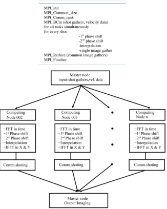
data, shot gathers, and parameters for wave extrapolation to each computing node by MPI_BCast. Each compu-ting node performs a wavefield extrapolation. After finishing extrapolation, the results are then sent to the mas-ter node by MPI_Reduce and then each single image gather is stacked for imaging subsurface. Figure 1 shows the basic flow chart for a parallel 3D PSPI algorithm.

4. Numerical Model Test

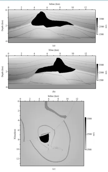
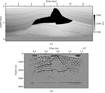
[image:4.595.152.479.245.654.2]

We conducted a numerical model test to verify prestack depth migration by the 3D PSPI. We applied it to the 3- D SEG/EAGE salt velocity model. The dimensions of the geological model are 10.8 km × 10.4 km × 4.2 km. The velocity range is 1500 m/s to 4482 m/s. Figure 2 shows the velocity model at inline 7760 m, xline 5320 m, and zline 1040 m, respectively. The grid size is Δx = Δy = Δz = 20 m and the number of grids is 541 × 521 × 211. The acquisition system consists of 8 streamers and each streamer has 68 receivers with 40 m distance. The

Table 1. A pseudo code for MPI_PSPI.

MPI_init

MPI_Common_size MPI_Comm_rank

MPI_BCat (shot gathers, velocity data) for all tasks simultaneously

for every shot

-1st _{phase shift}

-2nd _{phase shift}

-interpolation -single image gather MPI_Reduce (common image gathers) MPI_Finalize

(a)

(b)

[image:5.595.139.487.76.630.2]

(c)

Figure 2. Velocity model (a) at inline 7760 m, (b) xline 5320 m, and (c) zline 1040 m. The 3D velocity model shows geological interfaces, fault lines and saltbody. The highest velocity of the dark black is a saltbody.

Figure 3. Synthetic shotgaters at shot point number 30. Each shot gather has 68 receivers with 40 m distance.

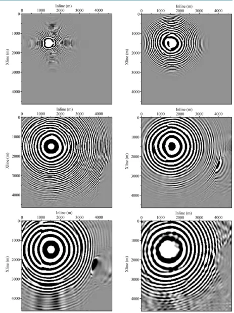
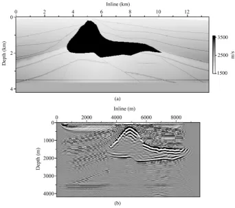
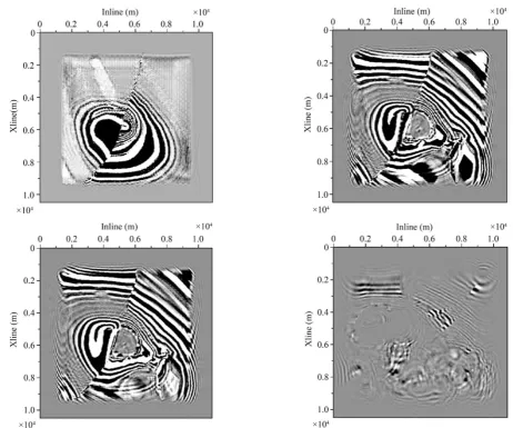
The prestack imaging by 3D PSPI entails extrapolation of wavefields in the wave number-frequency domain which are recorded on the surface, followed by finding wavefields at t = 0. A phase-shift was performed in the vertical and horizontal directions, respectively, and then interpolated at each node. This gave a single image gather according to the shot gather. After summation of every single image gather, we got a stacked image in depth domain. The results of wavefields extrapolation are shown in Figure 4. It shows extrapolated some parts of wavefields at 220 m, 1020 m, 1820 m, 2220 m, 3020 m, and 4020 m depth from top to bottom. We can see wavefields from the fault zone at 1020 m depth. Figure 5 shows the prestack migration results by 3D PSPI along the inline direction. The figures show the subsurface images on the inline axis. The top image is the result at inline 6360 m, which show some portions of the reflectors above the saltbody. The 2nd image is the resulting subsurface image for inline 7760 m, which shows some portions of the reflectors, the saltbody, and the reflectors of the subsalt. The 3rd and 4th images are the result at inline 9360 m and 10360 m. Figure 6 shows the compari-son of 3D velocity model and 3D PSPI image in depth domain at inline 7760 m. This shows the image of top saltbody is well imaged, but the geological interfaces of the lower parts of saltbody is poor. This means 3D PSPI is a good algorithm for fast velocity variations, but it would be limitation for imaging sub saltbody. Figure 7

shows the prestack migration results by 3D PSPI along the xline direction. These figures show the subsurface image along the xline direction. The top image is there sult at inline 1540 m, and shows the reflectors and the fault zone. The 2nd and 3rd images are the resulting subsurface image for xline 5320 m and 7540 m, which show some portions of the reflectors, the saltbody, and the reflectors of the subsalt. The 4th is the result at inline 8640 m. Figure 8 shows the comparison of the 3D velocity model and 3D PSPI at xline 5320 m. From the Figure 8

[image:7.595.78.542.77.698.2]

[image:8.595.80.539.80.361.2]

Figure 5. The results of 3D prestack depth migration at inline 6360 m, 7760 m, 9360 m, and 10,360 m from top to bottom. The images of the lower parts of saltbody are unclear due to a big velocity difference between the upper and the lower parts of saltbody.

(a)

(b)

[image:8.595.141.484.405.708.2]

[image:9.595.79.538.80.363.2]

Figure 7. The results of 3D prestack depth migration at xline 1540 m, 5320 m, 7540 m, and 8640 m from top to bottom. The results show fault lines and saltbody, but some geological interfaces of the lower parts of saltbody is uncelear.

(a)

(b)

[image:9.595.145.487.406.706.2]

[image:10.595.80.543.79.464.2]

Figure 9.The results of 3D prestack depth migration at zline 400 m, 1000 m, 1040 m, and 3000 m. The results show fault line and saltbody.

(a) (b)

[image:10.595.89.540.501.709.2]

5. Conclusion

Since 3D PSPI migration is efficient and requires less computation than RTM, it is a suitable tool for prestack depth migration, which requires heavy data input-output and huge computing time. We implemented 3D pres-tack depth migration on PSPI algorithm using Open MP and verified its performance on the synthetic 3D SEG/EAGE salt velocity model. The numerical model test shows that the results are in good agreement with the original geological model. The outline of saltbody is well imaged, but some geological interfaces of the lower parts of saltbody are poor. Though the numerical test shows reasonable results, for further study we need to per-form field data application to focus on developing a more elaborate velocity model. And, it also needs to devel-op an algorithm using GPU codes for fast more computation.

Acknowledgements

This work was supported by the Energy Efficiency & Resources Core Technology Program of the Korea Insti-tute of Energy Technology Evaluation and Planning(KETEP), granted financial resource from by the Ministry of Trade, Industry & Energy, Republic of Korea (No. 20132510100060).

References

[1] Gray, S.H. and May, W.P. (1994) Kirchhoff Migration Using Eikonal Equation Travel Times. Geophysics, 49, 124- 131. http://dx.doi.org/10.1190/1.1443639

[2] Bevc, D. (1997) Imaging Complex Structures with Semi-recursive Kirchhoff Migration. Geophysics, 62, 577-588.

http://dx.doi.org/10.1190/1.1444167

[3] Gray, S.H. (2005) Gaussian Beam Migration of Common Shot Records. Geophysics, 70, s71-s77.

http://dx.doi.org/10.1190/1.1988186

[4] Baysal, E., Kosloff, D. and Sherwood, J.W.C. (1983) Reverse Time Migration. Geophysics, 48, 1514-1524.

http://dx.doi.org/10.1190/1.1441434

[5] Liu, G., Liu, Y., Ren, L. and Meng, X. (2013) 3D Seismic Reverse Time Migration on GPGPU. Computers and Geos-ciences, 59, 17-23. http://dx.doi.org/10.1016/j.cageo.2013.05.009

[6] Loewenthal, D. and Mufti, I.R. (1983) Reversed Time Migration in Spatial Frequency Domain. Geophysics, 48, 627- 635. http://dx.doi.org/10.1190/1.1441493

[7] Whitmore, M.D. (1983) Iterative Depth Migration by Backward Time Propagation. The 53th Annual International Meeting,Society of Exploration Geophysics, Las Vegas, Expanded Abstract Session: S101.

http://dx.doi.org/10.1190/1.1893867

[8] Chattopadhyay, S. and McMechan, J. (2008) Imaging Condition for Prestack Reverse-Time Migration. Geophysics, 73, S81-S89. http://dx.doi.org/10.1190/1.2903822

[9] Gazdag, J. (1978) Wave Equation Migration with the Phase-Shift Method. Geophysics, 43, 1342-1351.

http://dx.doi.org/10.1190/1.1440899

[10] Stoffa, P.L., Fokkema, J.T., de Luna Freire, R.M. and Kessinger, W.P. (1990) Split-Step Fourier Migration. Geophysics,

55, 410-421. http://dx.doi.org/10.1190/1.1442850

[11] Gazdag, J. and Sguazzero, P. (1984) Migration of Seismic Data by Phase Shift plus Interpolation. Geophysics, 49, 124- 131. http://dx.doi.org/10.1190/1.1441643

[12] Bonomi, E., Brieger, L.M., Cazzola, L. and Zanoletti, F. (2006) Wavefield Migration plus Monte Carlo Imaging of 3D Prestack Seismic Data. Geophysical Prospecting, 54, 505-514. http://dx.doi.org/10.1111/j.1365-2478.2006.00557.x