Munich Personal RePEc Archive
Relative and Absolute Preference for
Quality
Angyridis, Constantine and Sen, Debapriya
Ryerson University
6 June 2010
Online at
https://mpra.ub.uni-muenchen.de/23103/
Relative and Absolute Preference for Quality
∗
Constantine Angyridis
†Debapriya Sen
‡June 6, 2010
Abstract
This paper seeks to explain two related phenomena: (i) it is often the case that when the new variety of a product is launched, some consumers do not purchase the latest variety and (ii) the quality of the latest variety of a product is often not significantly superior compared to the existing variety. We consider a simple model of monopoly with two types of consumers: “regular” (typeR) who cares only about theabsolutequality of the product and “fastidious” (type F) who cares about the relative quality vis-a-vis the existing variety. We show that it is never optimal for the monopolist to exclusively serve type F. Moreover, we identify situations where although it is optimal for the monopolist to upgrade the quality of the product, this upgrade is not sufficient to meet the standards of type F. As a result, only type R buys the upgraded variety while type F chooses not to buy it.
Keywords: Relative Preference, Absolute Preference, Singular Menu, Separating Menu
JEL Classification: D42, D82, D86, L15
∗For helpful comments, we are grateful to the seminar participants at California State University, Long
Beach; 2009 IMAEF conference, Ioannina and 2009 CEA meetings, Toronto.
†Department of Economics, Ryerson University, 380 Victoria Street, Toronto, ON, M5B 2K3, Canada.
Email: [email protected]
‡Corresponding author. Department of Economics, Ryerson University, 380 Victoria Street, Toronto,
1
Introduction
It is often the case that when a new variety of a product is launched, it does not receive a uniformly positive response from consumers. Some consumers do not buy the new variety as they do not consider it to be of significantly superior quality compared to the existing variety. There are two well known examples that validate these observations.
The first example involves the launching of “New Coke” by Coca Cola Co. on April 23, 1985. Despite a prolonged and aggressive advertising campaign, the public’s reaction to the new product was overwhelmingly negative. Soon people were stockpiling cases of the old Coke. According to Hartley (2006, p.34): “...by mid-May 1985 calls were coming in at the rate of 5,000 a day, in addition to a barrage of angry letters.” The Newsweek magazine reported in June 1985 that a case of the old Coke was sold in the black market for as much as $30. These events prompted Coca Cola to withdraw New Coke from shelves on July 11. Furthermore, company officials apologized to the public and brought back the old Coke in the market. Until this day, the launching of New Coke is widely considered to be one of the biggest marketing fiascoes in business history.1
The launching of the Operating System (OS) Windows Vista by Microsoft in early 2007 is another example. Many users did not consider Vista to be of significantly higher quality compared to the existing system Windows XP. The launching of Vista prompted the media outlet InfoWorld to set up the “Save XP” petition that was signed by more than 75,000 people by February 2008. A survey of 961 IT professionals conducted in late November 2007 found 90% of participants had major concerns about the new OS. The most important issue was the lack of stability of Vista relative to predecessor XP. According to InfoWorld,2
“...many businesses and consumers were not excited about dispensing their time and money upgrading to a new OS that they believe does not offer enough considerable advantages over XP, and are not keen on dealing with the incompatibility issues up-grading invariably causes. Their argument is simple—‘if it ain’t broke, don’t fix it’.”
These examples bring out an interesting aspect of consumer behavior: when the new variety of a product is launched, at least some consumers judge its quality not in absolute
terms, but rather in relative terms by comparing it with the existing variety. Accordingly, these consumers may not purchase the latest variety if the net quality improvement is not deemed to be sufficiently significant. This paper proposes a simple theoretical framework that models such consumer preference and seeks to provide an explanation of the cases described above.
Specifically, we consider a model of a product market that is served by a monopolist. The monopolist can produce an existing variety of low quality at zero cost. In addition, it can also produce a higher quality product by incurring additional costs. Each buyer in the market buys either one or zero unit of the good. The buyers are classified into two types according to the nature of their preference: typeR (regular) buyers care about theabsolute
quality of the product and typeF (fastidious) buyers care about itsrelative quality vis-a-vis the existing variety. The monopolist can offer either a single variety (singular menu) or a
1
Michael E. Ross, April 22, 2005. “New Coke and Other Marketing Fiascos,”MSNBC.com
http://www.msnbc.msn.com/id/7209828/
2
Andrew Hendry, February 6, 2008. “Microsoft responds to Save XP petition,”Computerworld
pair of varieties (separating menu) consisting of both the existing variety as well as a new variety of higher quality.
The nature of the preference of type F buyers plays a crucial role in our model. Indeed, this is the major point of departure from the existing literature that generally considers buyers who only care about the absolute quality of a product. When buyers care only about absolute quality (and there are two types), there is an exogenously fixed classification of buyers according to their willingness to pay for the product: “low type” and “high type”. In that case, regardless of the level of quality, high type buyers have a uniformly higher willingness to pay compared to low type. In contrast, there is no exogenously fixed low or high type in our model and whether a buyer is low or high type depends on the quality of the product. Type F is the high type if the new variety is of significantly superior quality compared to the existing variety, while typeR is the high type otherwise.
TypeRbuyers have a standard absolute preference for quality in our model. Accordingly, for typeRwe obtain the well known result that it is left with positive surplus in any optimal separating menu when it has a higher willingness to pay (see, e.g., Salani´e (2005)). This is not the case with type F. A type F buyer, having a relative preference for quality, never buys the existing variety. As a result, when a separating menu (i.e. a menu consisting of both the existing variety as well as a new variety of higher quality) is offered, the incentive compatibility constraint of type F is never binding. This enables the monopolist to charge the maximum possible price for the high-quality variety from type F to extract its entire surplus. Consequently, typeF is always left with zero surplus in any separating menu. Then it follows that it cannot be optimal for the monopolist to exclusively serve type F as by choosing a separating menu that serves both types, the monopolist can obtain additional profits from type R. Finally, we identify situations where it is optimal for the monopolist to offer a new variety exclusively for type R. The quality of this new variety, though higher than the existing level, is not significantly superior and as a result type F buyers do not buy it. This outcome closely resembles the examples of New Coke and Vista, where the new variety, though presumably superior, was not purchased by many consumers. To summarize our main results:
1. In any optimal separating menu, a type F buyer is always left with zero surplus, while a type R buyer may be left with positive surplus.
2. It is never optimal for the monopolist to exclusively serve type F buyers.
3. There are situations where it is optimal for the monopolist to offer a new variety of higher quality exclusively for type R buyers. Thus, although the monopolist offers a higher quality product, the quality improvement is not sufficiently significant to meet the standards of type F buyers and they do not buy the new product.
of some consumers to extract higher surplus from others (e.g., White (1977), Mussa and Rosen (1978), Maskin and Riley (1984)). Besanko et al. (1987) find in this regard that setting minimum quality standards may have ambiguous welfare implications as it may lead to exclusion of some consumers. Some recent papers include Kim and Kim (1996) who show that in the presence of spill-over effects in costs, higher willingness to pay may not necessarily lead to the provision of higher quality and it may be optimal for the monopolist to choose a pooling menu (i.e. only one price-quality pair). Acharyya (1998) argues that a separating menu may not be optimal without restrictions on cost functions and the extent of market coverage and moreover, there may not be any distortion on quality. Our result that it may be optimal for the monopolist to offer a pooling menu exclusively for type R is consistent with both Kim and Kim (1996) and Acharyya (1998). However, in contrast to these and other papers of the literature, the main driving force behind our results is the relative nature preference of type F buyers.
The monopoly model of this paper is arguably a reasonable approximation with respect to the examples of Coca Cola and Microsoft given before. For instance, Microsoft has continually enjoyed the lion’s share of the Operating System market over the past several years. According to the IT company NetApplications, Microsoft has maintained a market share of more than 90%.3 In the case of Coca Cola, its share in the Carbonated Soft Drinks
market may not be as dominant, but it is also quite significant. According to the magazine Beverage-Digest, the share of Coca Cola Co. in recent years is around 42% while its closest rival PepsiCo has a share of around 30%.4 From a theoretical viewpoint, the monopoly model
enables us to see the effect of relative preference in particular clarity. It is an important benchmark which can be extended to incorporate other relevant factors such as the effect of competition in the product market.
The paper is organized as follows. We present the model and derive the optimal price-quality schedules in Section 2. Section 3 endogenizes the choice of price-quality of the new variety. We conclude in Section 4. Most proofs are relegated to the Appendix.
2
The Model
Consider a good that is produced by a monopolistM.There is an existing variety of the good that has quality L > 0, which can be produced at zero cost. By incurring cost c(H) > 0, M can produce an additional variety of superior quality H > L. For this section, the level of superior quality H is considered to be exogenously given and we denote c(H) ≡ c. This assumption is relaxed in Section 3.
Any consumer in this market buys either one unit of the good or nothing. The market size is normalized to be 1, so each consumer can be viewed as a point in the interval [0,1].
A consumer can be either of the following two types: F (fastidious) and R (regular). Let
λ∈(0,1) denote the fraction of typeF consumers. The type presents the nature of preference for quality of a consumer. A type R consumer cares about the absolute quality of the good while a type F consumer cares about itsrelative quality vis-a-vis the existing quality L.For
X ∈ {L, H} and t∈ {R, F}, letvt(X) denote the valuation of a consumer of type t for the
3
Top Operating System Share Trend,Net Applications
http://www.netmarketshare.com/os-market-share.aspx?qprid=9
4
good of quality X. We assume that vR(X) = X and there is a constant θ > 1 such that
vF(X) =θ(X−L). That is,
vR(L) =L, vR(H) = H, vF(L) = 0 and vF(H) =θ(H−L) (1)
The specification in (1) captures the preferences of two types of consumers in a simple way. The valuation of type R is standard. Since type F cares about the relative quality, its valuation depends on the net quality improvement X−L rather than the absolute quality
X.The parameterθ > 1 captures the fact that type F is willing to pay more on the basis of the net quality improvement.5 To make this point precise, denote
τ(θ, L) :=θL/(θ−1) (2)
Observe that
vF(H) =θ(H−L)TvR(H) =H ⇔H Tτ(θ, L) (3)
This shows that the willingness of typeF to pay for qualityH is higher than the willingness of type R only when H is sufficiently high. Thus, if H ≥τ(θ, L), then type F is the “high type” and type R the “low type” while if H < τ(θ, L),the converse is true.
The product menu offered by M can be classified into the following categories, where
pX ≥0 stands for the price of qualityX:
(i) It is varied if it has two price-quality pairs h(L, pL),(H, pH)i. A varied menu is called
separating if it is optimal for type Rto buy a variety (X, pX) and it is optimal for type
F to buy a different variety (Y, pY).
(ii) It is singular if it has only one price-quality pair (X, pX) where X ∈ {L, H}.
Without loss of generality, we shall only consider singular and separating menus.
Consumers have separable utilities. A consumer who does not buy anything obtains zero utility. A type t consumer who buys variety X at price pX obtains utility vt(X)−pX.
2.1
Separating menus
When a separating menuh(L, pL),(H, pH)iis offered, a consumer of typethas three choices:
(i) buy (L, pL) to obtain vt(L)−pL or (ii) buy (H, pH) to obtain vt(H)−pH or (iii) buy
nothing and obtain zero. LetX, Y ∈ {L, H}and X 6=Y.A type t consumer buys (X, pX) if
and only if both of the following hold:
IRt(Individual rationality of type t): vt(X)−pX ≥0 (4)
ICt(Incentive compatibility of type t): vt(X)−pX ≥vt(Y)−pY (5)
Since vF(X) = θ(X−L), it follows by (4) that for any positivepL, vF(L) = 0 < pL, so type
F never buys variety L. Therefore, in order to determine the optimal menus for M in the
5
The valuations in (1) can have the following alternative interpretation. A type F consumer already purchased the variety of existing quality L in a previous period and as a result has a “reservation utility”
θL.If typeF switches to the variety of qualityH,it will obtainθH,so it comparesθHwithθL.In contrast, a typeR consumer is a first-time buyer of the product and has zero reservation utility, so typeRcompares
class of all separating menus, it is sufficient to consider menus where type R buys (L, pL)
and type F buys (H, pH). As the fraction of type F is λ, the cost of variety H is cand the
cost of L is zero, the profit of M from such a separating menu is
Π(pL, pH) =λ(pH −c) + (1−λ)pL (6)
By (1), (4) and (5),M’s problem is choosing pL, pH ≥0 to maximize Π(pL, pH) subject to
IRR(Individual rationality of type R): pL≤L
ICR(Incentive compatibility of typeR): H−pH ≤L−pL
IRF (Individual rationality of type F): pH ≤θ(H−L)
Constraint IRRimplies that buying (L, pL) is better for typeRthan buying nothing; similarly
IRF says that for type F, buying (H, pH) is better than buying nothing. Constraint ICR
says that for type R, buying (L, pL) is better than buying (H, pH). There is no incentive
compatibility constraint for type F since it never buys variety L.
Proposition 1 (Optimal separating menus) M has a unique optimal separating menu
h(L, pL),(H, pH)i that has the following properties.
(I) IRF always binds, i.e., pH =θ(H−L), so type F is always left with zero surplus.
(II) (Full Surplus Extraction(FSE))If H ≥τ(θ, L), IRR binds and type R is also left with
zero surplus. The optimal menu has pH = θ(H −L) and pL = L. M extracts full
surplus from both types to obtain λ[θ(H−L)−c] + (1−λ)L.
(III) (Partial Surplus Extraction(PSE))IfH < τ(θ, L), IRRdoes not bind and typeRis left
with positive surplus. The optimal menu haspH =θ(H−L)and pL =L−(H−pH) =
(θ−1)(H−L)< L. M extracts full surplus from type F and partial surplus from type
R to obtain λ[θ(H−L)−c] + (1−λ)(θ−1)(H−L).
(IV) ICR binds if H≤τ(θ, L) and it does not bind if H > τ(θ, L).
Proof See the Appendix.
An interesting conclusion is that typeF isalwaysleft with zero surplus under the optimal separating menu. One standard result in contract theory (see, e.g., Salani´e, 2005) is that under the optimal separating contract, the type that has a lower willingness to pay (“low type”) is left with zero surplus. In our model, a specific type does not have a uniformly lower willingness to pay for variety H. The low type is F if H < τ(θ, L), while it is R if
H ≥ τ(θ, L). Accordingly, type F obtains zero surplus if H < τ(θ, L) and type R obtains zero if H ≥ τ(θ, L), which is along the lines of the existing literature. The question is why is typeF left with zero surplus even whenH ≥τ(θ, L) (i.e. when it has a higher willingness to pay)? The reason is that as type F never buys varietyL, M has the opportunity to raise
pH to the highest level possible without facing the risk that F will switch to varietyL. This
2.2
Singular menus
When a singular menu (X, pX) is offered, a consumer of type t has two choices: (i) to buy
the menu to obtain utility vt(X)−pX or (ii) to not buy at all and obtain zero. Therefore a
type t consumer buys if and only if
IRt(Individual rationality of type t): vt(X)−pX ≥0 (7)
By (1) and (7), the optimal choices of consumers for singular menus are
(i) (L, pL): Type F never buys and type R buys iffpL≤L.
(ii) (H, pH): Type F buys iff pH ≤θ(H−L) and typeR buys iff pH ≤H.
Note by (2) that
θ(H−L)TH ⇔H Tτ(θ, L) (8)
Therefore, for a menu (H, pH),we have
(a) If H ≥ τ(θ, L), both types buy the menu when pH ≤ H, only type F buys when
H < pH ≤θ(H−L) and no one buys whenpH > θ(H−L).
(b) IfH < τ(θ, L),both types buy the menu whenpH ≤θ(H−L), only type Rbuys when
θ(H−L)< pH ≤H and no one buys when pH > H.
Proposition 2 (Optimal Singular Menus)
(I) Consider the set SL = {(L, pL)|pL ≥ 0} of all singular menus where M offers only
variety L. The optimal menu over this set has pL = L where type R is left with zero
surplus, type F does not buy and M obtains (1−λ)L.
(II) Consider the set SH = {(H, pH)|pH ≥ 0} of all singular menus where M offers only
variety H. The optimal menu over this set has the following properties.
(a) For H ≥τ(θ, L):
(i) If c≥θ(H−L), M does not obtain positive profit from any menu in SH.
(ii) If H ≤ c < θ(H−L), M sets pH =θ(H −L). Type R does not buy, type F
buys and is left with zero surplus and M obtains λ[θ(H−L)−c]>0.
(iii) If c < H, ∃ λ(H)≡(H−c)/[θ(H−L)−c] such that
• If λ > λ, M sets pH = θ(H −L); type R does not buy, type F buys and
is left with zero surplus and M obtains λ[θ(H−L)−c]>0.
• If λ≤λ, M sets pH =H; both types buy, type R is left with zero surplus,
type F with positive surplus and M obtains H−c >0.
(b) For H < τ(θ, L) :
(i) If c≥H, M does not obtain positive profit from any menu in SH.
(ii) If θ(H−L)≤c < H, M sets pH =H. TypeF does not buy, type R buys and
(iii) If c < θ(H−L), ∃ λ∗(H)≡[H−θ(H−L)]/(H−c) such that
• If λ > λ∗, M sets p
H =θ(H−L); both types buy, type F is left with zero
surplus, type R with positive surplus and M obtains θ(H−L)−c >0.
• If λ ≤λ∗, M sets p
H =H; type F does not buy, type R buys and is left
with zero surplus and M obtains (1−λ)(H−c)>0.
Proof See the Appendix.
2.3
Optimal menus
Having identified optimal menus for M in two different classes, separating (Prop 1) and singular (Prop 2), now we are in a position to characterize globally optimal menus for M.
Towards this end, we begin with Lemma 1, which is also of some independent interest.
Lemma 1 Offering a singular menu exclusively for type F can never be a globally optimal choice for M.
Proof We know that type F will never buy a singular menu that has variety L,so consider a singular menu (H, pH) that is offered exclusively for type F. If this menu is optimal for
M, then by Prop 2(II), we must have H ≥ τ(θ, L) and pH = θ(H −L) that gives M the
profit Π(θ(H −L)) = λ[θ(H−L)−c]. By Prop 1(II), if H ≥ τ(θ, L), then M obtains
λ[θ(H−L)−c] + (1−λ)L >Π(θ(H−L)) from its optimal separating menu, so the singular menu (H, θ(H−L)) cannot be globally optimal.
The lemma above shows that it is never optimal for M to exclusively serve type F (the type that cares about relative quality). To see the intuition, first note that when variety
H is not of significantly superior quality (H < τ(θ, L)), type F is willing to pay less than type R. In this case, type R is the high type and it is clear that it must be served in any singular menu that exclusively serves one type. In contrast, if variety H is of significantly superior quality (H ≥τ(θ, L)), then it may be optimal forM to offer an exclusive menu for typeF and extract the entire surplus from this type. However, we have seen in Proposition 1 that due to the relative preference of type F, the monopolist always extracts the entire surplus fromF in its optimal separating menu. Consequently, it is better for the monopolist to choose this separating menu as it enablesM to obtain additional profits from type R.
In view of Proposition 2 and Lemma 1, in our search for optimal menus, it is sufficient to compare optimal separating menus from Proposition 1 with:
(i) Low quality exclusive (LQE) menu for type R: pL=L and M obtains (1−λ)L.
(ii) High quality exclusive (HQE) menu for typeR: pH =H and M obtains (1−λ)(H−c).
(iii) High quality inclusive (HQI) menu: both types buy. If H ≥ τ(θ, L), then pH = H,
type R is left with zero surplus, type F with positive surplus and M obtains H −c. If H < τ(θ, L), then pH = θ(H −L), leaving type F with zero surplus, type R with
positive surplus and M obtains θ(H−L)−c.
Proposition 3 The optimal menus of M are given as follows.
(II) If c < θ(H−L) and H ≥τ(θ, L):
(a) For H−L≤c < θ(H−L), it is the FSE separating given in Prop 1.
(b) For c < H−L, ∃ bλ(H)∈(0,1) such that
(i) if λ >bλ, it is the FSE separating menu given in Prop 1.
(ii) if λ ≤bλ, it is the HQI menu with pH =H and M obtains H−c.
(III) If c < θ(H−L) and H < τ(θ, L), ∃ λ∗(H) ≡ [H−θ(H−L)]/(H−c) ∈ (0,1) such
that
(a) For H−L≤c < θ(H−L):
(i) if λ > λ∗, it is the PSE separating menu given in Prop 1.
(ii) if λ ≤λ∗, it is the LQE menu with p
L=L and M obtains (1−λ)L.
(b) For c < H−L:
(i) ifλ > λ∗,it is the HQI menu withpH =θ(H−L)andM obtainsθ(H−L)−c.
(ii) if λ ≤λ∗, it is the HQE menu with pH =H and M obtains (1−λ)(H−c).
Proof See the Appendix.
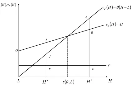
To see the intuition for the results of Proposition 3, first observe that if c≥ θ(H−L), it is prohibitively expensive for M to produce variety H, so it chooses only variety L to exclusively serve type R (Prop 3(I)). If c < θ(H−L), it is potentially worthwhile for M to produce H and its optimal menu depends on the threshold τ(θ, L) (Prop 3(II)-(III)). This threshold captures the degree of superiority of H relative to the existing variety L. Figure 1 presents the valuations of two types vR(H) and vF(H) and using (3), identifiesτ(θ, L) as
the point of intersection of these two functions.
If H ≥ τ, variety H is of significantly superior quality, so that type F buyers have a higher willingness to pay for H.For this case, F is the high type andR the low type. In the optimal separating menu, typeR buysLand the monopolist sets a large price for varietyH
to extract full surplus from typeF (FSE menu, Prop 1(II)). Alternatively, M has the option of offering a singular menu consisting of only varietyH where both types buy (HQI menu). The price ofH here has to be lower than the corresponding price in the FSE menu to induce the low type (type R) to buy. The trade-off between setting a high price of H where only typeF buys H (FSE) and a lower price where both types buy H (HQI) is settled by costc
as well as the relative fractions of the two types in the market.
To see this, consider an arbitrary H ≥τ, given by H′ in Figure 1. The monopolist can
either offer H to type F and L to type R by setting pH = AH′ and pL = OL (FSE), or it
can offer H to both types by setting pH = BH′ (HQI). If it switches from FSE to HQI, it
incurs the loss λAB from type F and gains (1−λ) (BH′ −c−OL) = (1−λ) (BE −OL)
from type R. If c is large (c ≥ H −L), BE is small, causing M to choose the FSE menu (Prop 3(II)(a)). If c < H −L, BE is large and provided that the fraction of typeR is also large (λ ≤λb), it is optimal for M to choose the HQI menu. Otherwise (λ >bλ), it is optimal to still choose the FSE menu (Prop 3(II)(b)).
Figure 1: vF(H), vR(H) and τ(θ, L)
previous case. However, there is an important difference. Since the high type of the previous case (typeF) had a relative preference, it never boughtL,enablingM to extract full surplus from both types in its optimal separating menu (Prop 1(II)). However, for the present case, the high type (type R) has an absolute preference and in the optimal separating menu it has to be left with positive surplus (Prop 1(III)). For this reason, the separating menu loses some of its appeal for H < τ, as evident by comparing parts (II) and (III) of Proposition 3. To see the intuition for the results of Prop 3(III), consider an arbitrary H < τ given by H′′ in Figure 1. The monopolist can either offer variety H to type F (the low type) by
setting pH =JH′′, or it can setpH =IH′′ > JH′′ to serve only R and exclude F.
When the fraction of F is large (λ > λ∗), it is optimal for M not to exclude type F
(Prop 3(III)(a)(i),(b)(i)). Regarding type R, M has two options. It can offer only varietyH
at pH = JH′′ so that both types buy H and type R is left with surplus IH′′−JH′′ =IJ
(HQI menu) or it can offer L at pL = OL−IJ for type R, making R indifferent between
the two varieties, so that R buys L and F buys H (PSE menu). If M switches from HQI to PSE, it incurs the loss (1−λ) (JH′′−c) = (1−λ)JK and gains (1−λ) (OL−IJ) from
3(III)(b)(i)).
When the fraction of F is small (λ ≤ λ∗), it is optimal for M to exclude type F and
serve type Rexclusively (Prop 3(III)(a)(ii),(b)(ii)). In particular, it is not optimal to offer a separating menu for this case. M can either offer varietyH atpH =IH′′(HQE) or varietyL
atpL=OL(LQE). If M switches from HQE to LQE, it incurs the loss (1−λ) (IH′′−c) =
(1−λ)IK and gains (1−λ)OL. As before, for higher levels of c, IK is sufficiently small resulting in M choosing the LQE menu (Prop 3(III)(a)(ii)), while for lower levels of c, it is optimal to choose the HQE menu (Prop 3(III)(b)(ii)).
The last part of Proposition 3 ((III)(b)(ii)) is of particular interest as it connects our model with the motivating examples of Windows Vista and New Coke. It identifies situ-ations where the monopolist offers a new variety of superior quality H, but a segment of consumers (type F) does not to buy it. This result is driven by the relative preference of type F consumers. Comparing the quality of the new variety H in relation to the existing level L, they find the quality improvement not sufficiently significant to meet their stan-dards. Accordingly, they are not willing to pay much for variety H, which drives M to offer H exclusively for type R. Observe that offering such an HQE menu is optimal for M
only when the fraction of type F is small in the market (λ ≤ λ∗). Regarding Microsoft’s
launching of Vista, it can be argued that although many consumers found Vista to be not of significantly superior quality in relation to the existing system XP, these consumers still possibly constituted only a small segment of the market. Given that, Microsoft might have found it optimal to launch an upgrade that was only moderately superior and excluded this segment in the process. The case of launching of New Coke is different where Coca Cola was eventually compelled to withdraw the new product from the market. From the description of the events following the launching of New Coke, it is evident that most consumers were strongly attached to the existing variety of Coke, suggesting a relative nature of preference for these consumers. Therefore, one plausible explanation of the New Coke fiasco could be the failure on part of Coca Cola to recognize that a very large segment of its consumers had a relative preference.
3
Endogenous
H
The level of the superior quality H was considered to be exogenously given in the last section. For any such exogenous H, we characterized optimal menus in Proposition 3. In this section we address the issue of whether our conclusions are robust when the choice ofH
is endogenous, i.e., when M can choose any H > L rather than an exogenously given level. Instead of characterizing the optimal menus under endogenousHfor all possible values of the parameters of the model, for clarity of presentation we shall focus on the primary motivating question of this paper: when M can choose any H > L, are there situations where it finds it optimal to choose a level of H where only type R buys the new variety and type F is excluded? We shall identify sufficient conditions on the parameters of the model where this will be case.
We endogenize the choice of H by allowing M to produce a variety of superior quality of any levelH > L. The production cost c(H) is assumed to be increasing and convex, with
c(L) = 0.Specifically, we assume that
The parameter α captures how costly it is to produce a high quality good. Denote
e
H ≡L+ 1/α and H ≡L+θ/α (10)
Since α >0 and θ >1,we have L <H < H.e Note from (9) that
c(H)< H −L if H ∈(L,He], H −L≤c(H)< θ(H−L) ifH ∈[H, He )
and c(H)≥θ(H−L) if H ≥H (11)
Using (11) in Prop 3(I), for H ≥ H, the optimal menu is the LQE menu (L, L) where M
obtains (1−λ)L. Therefore, the profit of M is invariant of H for H ≥H and to determine optimalH, it is sufficient to consider H ∈[L, H]. Comparing τ(θ, L) =θL/(θ−1) andH,
τ(θ, L)TH⇔θ Sθ where θ(α, L) := (1 +√1 + 4αL)/2 (12)
Note that if θ < θ, then H < τ(θ, L) for all H ∈ [L, H] (by (11), c(H) ≤θ(H−L) in this interval). In that case, part (III) of Prop 3 applies, where the optimal menus depend on whether or not λ < λ∗(H). Using (9), we have
λ∗(H) = [H−θ(H−L)]/[H−c(H)] = [H−θ(H−L)]/[H−α(H−L)2] (13)
Lemma 2If θ < θ, then
(i) H < τ(θ, L), H > θ(H−L), H > c(H) for all H ∈[L, H].
(ii) λ∗(H) is well defined and positive for all H ∈[L, H] and λ∗(L) =λ∗(H) = 1.
(iii) ∃ H ∈(L, H)such that λ∗(H) is decreasing for H ∈[L, H), increasing for H ∈(H, H]
and attains its minimum at H =H.
(iv) ∃ θ < θe given by eθ(α, L) := (2αL+ 1)/(αL+ 1) such that H SHe ⇔θ Sθ.e
(v) If θ <θ,e then the profit of M is either constant or decreasing for H ≥H.e
Proof See the Appendix. Denote
HE ≡L+ 1/2α and HI ≡L+θ/2α (14)
Observe thatL < HE < HI.
Proposition 4 Let θ < eθ.There is eλ(θ, α, L)∈(0,1)such that
(i) If λ >eλ, the optimal menu forM is the HQI menu with H =HI and pH =θ(HI−L).
Both types buy and M obtains θ(HI−L)−c(HI) =θ2/4α.
(ii) If λ ≤λ,e the optimal menu for M is the HQE menu with H =HE andpH =HE. Only
Proof See the Appendix.
Proposition 4 identifies situations (θ < θe) such that if the fraction of type F in the market is small (λ ≤ λe), then although M finds it optimal to upgrade its product from existing quality L to a superior quality HE > L, this upgrade is not significant to meet the
standards of type F.As a result, only typeRbuys the new variety while typeF is excluded. However, if the fraction of type F is large (λ >eλ), then it is optimal for M to upgrade its product to a higher level of quality HI > HE. Such a quality improvement is sufficiently
significant so that both types F and R buy the new variety. It can be also noted that when
λ ≤λ,e the quality of the new variety HE is independent of θ (the parameter that captures
the willingness to pay for type F). However, whenλ >eλ, the upgraded quality HI depends
onθ and both the quality and the profit of M is monotonically increasing inθ.
To see the economic interpretation of the sufficient conditionθ <θ,e observe from Lemma 2 that θeis increasing in αL. Thus, an implication of the conditionθ < eθ is that either α is large (i.e. it is costly to produce a high quality variety) or L is large (i.e. the quality of the existing variety is quite good). The parameterα simply captures the cost effect. The role of the parameter L is more interesting: with large L, the effect of relative preference becomes more dominant, because when the existing variety is already of reasonably good quality, it becomes more difficult to meet the standards of typeF.
4
Concluding remarks
This paper provides a simple theoretical framework to understand two related phenomena: (i) when the new variety of a product is launched, some buyers are reluctant to purchase the latest variety and (ii) the quality of the new variety of a product may not be significantly superior compared to its previous version. We consider a monopoly model with two types of buyers who differ in terms of the nature of their preference: one type cares about the absolute quality of a variety (type R), while the other type cares about its relative quality (type F). We show that type F is always left with zero surplus in any optimal separating menu (Proposition 1) and it is never optimal for the monopolist to exclusively serve type
F (Lemma 1). Then we identify situations where it is optimal for the monopolist to offer a high quality variety exclusively for type R (Proposition 3). Furthermore, we show that when the quality choice is endogenous, the quality of the upgraded product is responsive to the preference of type F consumers only when they constitute a substantial segment of the market. Otherwise, it is optimal for the monopolist to only carry out incremental improvements in quality that results in typeF consumers not buying the upgraded product (Proposition 4).
Appendix
Proof of Proposition 1(I): Consider a menu where IRF does not bind, i.e. pH < θ(H−L).
If IRR also does not bind (pL< L), thenM can choose a new menu where the prices of both
varieties are raised to pL+ε and pH +ε with ε > 0 sufficiently small. For the new menu
ICR will continue to hold, while both IRR and IRF will hold for small values of ε. As ε >0,
M’s profit in the new menu is higher, so the old menu cannot be optimal.
Now consider a menu where IRF does not bind, but IRR does (pL=L.) UsingpL=Lin
ICR, we have pH ≥H. Observe by (2) that if H < τ(θ, L), then θ(H−L)< H, so it is not
possible to have both pH < θ(H−L) and pH ≥ H. Consider H ≥ τ(θ, L), which implies
that H ≤θ(H−L). HavingpH ∈[H, θ(H−L)) cannot be optimal for M as it can raisepH
to improve its profit. This proves that an optimal menu must have pH =θ(H−L).
(II)-(IV): Taking pH = θ(H −L) in (6), the problem of M reduces to choosing pL to
maximize (1−λ)pL subject to (a)pL≤L(IRR) and (b)pL ≤(θ−1)(H−L) (ICR). Clearly,
it is optimal forM to choose pL= min{L,(θ−1)(H−L)}.Noting that
(θ−1)(H−L)SL⇔H Sτ(θ, L),
it follows that if H ≥ τ(θ, L), then M chooses pL = L ≤ (θ − 1)(H − L) that binds
IRR (and does not bind ICR except if H = τ(θ, L)). If H < τ(θ, L), then M chooses
pL = (θ −1)(H − L) < L that binds ICR, but where IRR does not bind. This proves
(II)-(IV).
Proof of Proposition 2(I): Follows immediately by noting that typeF never buys variety
L and typeR buys (L, pL) only if pL ≤L.
(II): Observe that when menu (H, pH) is offered, typeR buys only ifpH ≤H while type
F buys only if pH ≤θ(H−L).
(II)(a) By (2),if H ≥τ(θ, L),then H ≤θ(H−L).IfpH > θ(H−L),then no type buys
and M obtains zero. If H < pH ≤θ(H−L), then only type F buys; over this interval, it is
optimal for M to set pH = θ(H−L) that gives it profit Π(θ(H −L)) = λ[θ(H−L)−c].
Finally, if pH ≤ H, then both types buy; over this interval, it is optimal for M to set
pH =H where type R is left with zero surplus, type F with positive surplus and M obtains
Π(H) =H−c.
(i) If c≥θ(H−L)≥H,both Π(θ(H−L)) and Π(H) are at most zero which proves (i). (ii) If H ≤c < θ(H−L), then Π(H)≤0<Π(θ(H−L)) which proves (ii).
(iii) If c < H, then both Π(H) and Π(θ(H−L)) are positive and (iii) follows by noting that Π(θ(H−L)TΠ(H)⇔λTλ.
(II)(b) By (2), if H < τ(θ, L), then H > θ(H−L). If pH > H, then no type buys and
M obtains zero. If θ(H −L) < pH ≤ H, then only type R buys; over this interval, it is
optimal forM to setpH =H that gives it profit Π(H) = (1−λ) [H−c]. IfpH ≤θ(H−L),
then both types buy; over this interval, it is optimal for M to set pH = θ(H−L) where
type F is left with zero surplus and type R is left with positive surplus. M obtains profit Π(θ(H−L)) = [θ(H−L)−c].
(iii) If c < θ(H−L), then both Π(H) and Π(θ(H−L)) are positive and (iii) follows by noting that Π(H)TΠ(θ(H−L))⇔λSeλ.
Proof of Proposition 3 We determine globally optimal menus by comparing the profit of M from (i) the optimal separating menu, (ii) the optimal (singular) menu over SH =
{(H, pH)|pH ≥ 0} and (iii) the optimal (singular) menu over SL = {(L, pL)|pL ≥ 0}. The
nature of the menu appears as superscripts in the profit of M. By Prop 2(I), the optimal menu over SL is the LQE menu with pL =L where M obtains ΠLQEλ = (1−λ)L >0.
(I) Let c≥ θ(H−L). If H ≥ τ(θ, L), then by Prop 1(II), the optimal separating menu is the FSE menu and
ΠFSEλ ≤(1−λ)L= Π
LQE
λ
If H < τ(θ, L), then by Prop 1(III), the optimal separating menu is the PSE menu and
ΠPSEλ ≤(1−λ)(θ−1)(H−L)<(1−λ)L= Π
LQE
λ
since for this case, (θ−1)(H−L)< L(by (8)). Thus, it is sufficient to compare LQE with the optimal menu overSH.
If eitherH ≥τ(θ, L) orH < τ(θ, L) and c≥H,then no menu inSH gives positive profit
(Prop 2(II)(a)(i),(b)(i)), so LQE is optimal. Finally let H < τ(θ, L) and c < H. Then by Prop 2(II)(b)(ii), the optimal menu over SH gives profit
(1−λ)(H−c)≤(1−λ)[H−θ(H−L)]<(1−λ)L= ΠLQEλ
since c≥θ(H−L) and θ >1. This proves the optimality of LQE.
(II) Let c < θ(H−L) andH ≥τ(θ, L).Then by Prop 1(II), the optimal separating menu is the FSE menu where M obtains
ΠFSEλ =λ[θ(H−L)−c] + (1−λ)L >(1−λ)L= Π
LQE
λ
So for this case it is sufficient to compare FSE with the optima menu over SH.
If either H ≤c < θ(H −L) or c < H and λ≥ λ, then the optimal menu over SH gives
profit λ[θ(H −L)−c] (Prop 2(II)(a)(ii),(iii)), which is less than ΠFSEλ . So let c < H and
λ < λ. Then the optimal menu over SH is the HQI menu with pH =H and ΠHQI =H−c
(Prop 2(II)(b)(iii)). Let
∆(λ) := ΠFSEλ −ΠHQI =λ[θ(H−L)−H]−(1−λ)(H−L−c) (15)
Since H ≥ τ(θ, L), by (8), θ(H −L) ≥ H. Thus, if c ≥ H −L, then ∆(λ) ≥ 0 and the optimal menu is the FSE menu, proving part (II)(a).
To prove (b), let c < H−L.Then ∆′(λ) = [θ(H−L)−H] + (H−L−c)>0.Note from
Prop 2(II)(a)(iii) that when λ = λ(H), ΠHQI = H−c =λ[θ(H−L)−c], so that ∆(λ) = (1−λ)L > 0. Since g(0) = −(H−L−c) <0, it follows that ∃ bλ(H) ∈ (0, λ(H)) ⊂ (0,1) such that ∆(λ)T0⇔λTλ. This proves (II)(b).
(III) Let c < θ(H−L) and H < τ(θ, L). Then the optimal separating menu is the PSE menu (Prop 1(III)) where M obtains
In the class of singular menus, the optimal menu is either LQE or HQI with pH =θ(H−L)
or HQE with pH =H (Prop 2(II)(b)(iii)). Note that
ΠLQE = (1−λ)L,ΠHQI =θ(H−L)−cand ΠHQEλ = (1−λ)(H−c)
We observe that
ΠHQEλ −Π
LQE
λ = ΠHQI−ΠPSEλ = (1−λ)(H−L−c) (16)
By (16), ΠHQI−ΠHQEλ = ΠPSEλ −Π
LQE
λ .Noting by Prop 2(II)(b)(ii) that ΠHQI TΠ
HQE
λ ⇔
λTλ∗, we conclude
ΠHQI TΠHQEλ ⇔ΠPSEλ TΠ
LQE
λ ⇔λ Tλ∗ (17)
To prove (III)(a), let H − L ≤ c < θ(H − L). Then by (16), ΠLQEλ ≥ Π
HQE
λ and
ΠPSEλ ≥ ΠHQI. If λ≥ λ∗, then by (17), Π
HQE
λ ≤ ΠHQI ≤ ΠPSEλ and Π
LQE
λ ≤ΠPSEλ . Hence
for this case, the optimal menu is PSE, proving part (III)(a)(i). If λ < λ∗, then by (17),
ΠHQI < ΠHQEλ ≤ Π
LQE
λ and ΠPSEλ < Π
LQE
λ , so for this case, the optimal menu is LQE,
proving part (III)(a)(ii).
For (III)(b), let c < H−L. Then by (16), ΠLQEλ <Π
HQE
λ and ΠPSEλ <ΠHQI.If λ≥λ∗,
then by (17), ΠHQI ≥ ΠHQEλ >ΠLQE. Since ΠHQI >ΠPSEλ , for this case the optimal menu
is HQI, proving part (III)(b)(i). If λ < λ∗, then by (17), ΠHQE
λ > ΠHQI > ΠPSEλ . Since
ΠHQEλ >Π
LQE
λ ,for this case, the optimal menu is HQE, proving part (III)(b)(ii).
Proof of Lemma 2 (i) If θ < θ, then by (12), H < τ(θ, L). So for all H ∈[L, H],we have
H < τ(θ, L). Then by (8), H > θ(H−L). Since c(H) ≤θ(H−L) for H ∈ [L, H], we have
H > c(H).
(ii) The first part is immediate from (i). As c(L) = 0 andc(H) = θ(H−L), the last part follows from (13).
(iii) Let λ∗
1(H)≡dλ∗(H)/dH. Note that
λ∗
1(H)T0⇔g(H)T0 whereg(H) :=α(H−L)[(1 +θ)L−(θ−1)H]−θL (18)
As g′(H) = 2α(θ−1)(τ(θ, L)−H) > 0, g(H) is monotonic for all H ∈ [L, H]. As g(L) =
−θL <0 andg(H) = θ(θ−1)[τ(θ, L)−H]>0,∃H ∈(L, H) such thatg(H)T0⇔H TH
which proves (iii).
(iv) As g(He) = (1 +αL)(θe−θ)/α,it follows that λ∗
1(He)T0⇔θ Seθ.Then (iv) follows
from (iii).
(v) We know that the profit ofM is a constant forH ≥H,so considerH ∈[H, He ].Then by (11),H−L≤c(H)≤θ(H−L) and Prop 3(III)(a) applies.
First suppose H∈[H, He ] andλ < λ∗(H).Then by Prop 3(III)(a)(ii), it is best for M to
choose the LQE menu that yields profit (1−λ)L which does not depend on H.
Next suppose H ∈[H, He ] andλ≥λ∗(H).Since θ >θ,e we haveH > He (part (iv)), so by
By Prop 3(III)(a)(i), for this case it is best for M to choose the PSE menu given in Prop 1 that yields profit
π(H) = λθ(H−L)−α(H−L)2+ (1−λ)(θ−1)(H−L)
Asπ(H) is strictly concave andπ′(He) =θ−1−λ≤θ−1−λ∗(He) =−(2αL+1)(θb−θ)/αL <0,
it follows that π(H) is decreasing for allH ∈[H, He ].
Proof of Proposition 4 Let θ < eθ. By Lemma 2(v), in search for optimal menus, it is sufficient to consider H ∈ [L,He], where c(H)≤H−L (by (11)). Since θ <θ < θ,b we have
H < τ(θ, L) for all H ∈ [L,He] (Lemma 2(i)). So we can use the results of (III)(b) of Prop 3, where for any H, the optimal menu depends on whether or not λ > λ∗(H). Denote
Aλ :={H ∈[L,He]|λ≤λ∗(H)} and Aλ :={H ∈[L,He]|λ≥λ∗(H)}
Case 1 H ∈Aλ: By Prop 3(III)(b), the best menu is the HQE menu where M obtains the
profit
ΠHQEλ (H) = (1−λ)[H−c(H)] = (1−λ)[H−α(H−L)
2] (19)
Observe that ΠHQEλ (H) is increasing for H < HE, decreasing for H > HE and its unique
unconstrained maximum is attained at HE whereHE ≡L+ 1/2α∈(L,He).
If λ ≤λ∗(HE), then HE ∈ Aλ and it is the optimal choice over H ∈Aλ. If λ > λ∗(HE),
then HE ∈/ Aλ and any optimal choice over H ∈ Aλ has λ∗(H) = λ, making such a choice
feasible for H ∈Aλ.
Case 2 H ∈Aλ: By Prop 3, the best menu is the HQI menu that yields the profit
ΠHQI(H) =θ(H−L)−c(H) =θ(H−L)−α(H−L)2 (20)
Let HI := L+θ/2α > L. Since θ < bθ < 2, we have HI < He = L+ 1/α. We note that
ΠHQI(H) is increasing for H < HI, decreasing for H > HI and its unique unconstrained
maximum is attained atHI.
We observe thatHI > HE and from the conditionθ > bθ,it follows thatλ∗(HE)> λ∗(HI).
For λ∈[0, λ∗(HI)], HE ∈Aλ and HI ∈/ Aλ, so the global optimal choice is HE (HQE menu
with H =HE). Forλ ∈[λ∗(HE),1], HI ∈ Aλ and HE ∈/ Aλ, so the global optimal choice is
HI (HQI menu with H =HI).
Finally consider λ ∈ [λ∗(HI), λ∗(HE)]. Then HE ∈ Aλ and HI ∈ Aλ. Since HE is the
unique maximizer of (19) and HI the unique maximizer of (20),
ΠHQEλ (HE)>ΠHQEλ (HI) and ΠHQI(HI)>ΠHQI(HE) (21)
Recall by Prop 3(III)(b) whenλ =λ∗(H) for some H, HQE and HQI menus yield the same
profit under that H,so that
ΠHQEλ∗(HI)(HI) = Π
HQI(H
I) and ΠHQEλ∗(HE)(HE) = Π
HQI(H
E) (22)
Denote ∆λ := ΠHQI(HI)−ΠHQEλ (HE).As both HE and HI are independent ofλ, from (19)
and (20), ∆λ is increasing in λ. From the first inequalities of (21) and (22), ∆λ∗(HI) < 0
and from the last inequalities, ∆λ∗(HE) > 0. Therefore, ∃ λe ∈ (λ∗(HI), λ∗(HE)) such that
∆λ T 0 ⇔ λ T λ.e This proves that the HQI menu with H = HI is optimal for λ > eλ and
References
Acharyya, R. 1998. Monopoly and Product Quality Separating or Pooling Menu? Economics Letters, Vol. 61, 187-194.
Besanko, D., Donnenfeld, S. and White, L.J. 1987. Monopoly and Quality Distortion: Effects and Remedies. Quarterly Journal of Economics, Vol. 102, 743-768.
Kim, J.-H. and Kim, J.-C. 1996. Quality Choice of a Multiproduct Monopolist and Spill-over Effect. Economics Letters, Vol. 52, 345-352.
Maskin, E. and Riley, J. 1984. Monopoly with Incomplete Information. Rand Journal of Economics, Vol. 15, 171-196.
Mussa, M. and Rosen, S. 1978. Monopoly and Product Quality. Journal of Economic Theory, Vol. 18, 301-317.
Hartley, R.F. 2006. Marketing Mistakes and Successes, John Wiley & Sons Inc.
Salani´e, B. 2005. The Economics of Contracts: A Primer. The MIT Press, Cambridge, Massachusetts.
Spence, A.M. 1975. Monopoly, Quality and Regulation. Bell Journal of Economics, Vol. 6, 417-429.