The Timing of Daily Demand for Goods
and Services – Multivariate Probit
Estimates and Microsimulation Results
for an Aged Population with German
Time Use Diary Data
Merz, Joachim and Hanglberger, Dominik and Rucha, Rafael
Forschungsinstitut Freie Berufe (FFB)
March 2009
Online at
https://mpra.ub.uni-muenchen.de/16303/
FFB
Forschungsinstitut
Freie Berufe
Fakultät II - Wirtschafts-, Verhaltens- und Rechtswissenschaften
Postanschrift:
Forschungsinstitut Freie Berufe Postfach 2440
21314 Lüneburg
[email protected] http://ffb.uni-lueneburg.de Tel: +49 4131 677-2051 Fax:+49 4131 677-2059
The Timing of Daily Demand for Goods and Services –
Multivariate Probit Estimates and Microsimulation Results for an
Aged Population with German Time Use Diary Data
Joachim Merz, Dominik Hanglberger and Rafael Rucha
The Timing of Daily Demand for Goods and Services –
Multivariate Probit Estimates and Microsimulation Results
for an Aged Population with German Time Use Diary Data
Joachim Merz, Dominik Hanglberger and Rafael Rucha1
FFB-Discussionpaper No. 77
March 2009 ISSN 0942-2595
1
Univ.-Prof. Dr. Joachim Merz, Dipl.-Volksw. Dominik Hanglberger, Dipl.-Volksw. Rafael Rucha, Research Institute on Professions (Forschungsinstitut Freie Berufe, FFB), Chair ‘Statistics and Professions’, Faculty II – Economic, Behavioural and Law Sciences, Leuphana University of Lüneburg, Campus: Scharnhorststr. 1, Geb. 5, 21332 Lüneburg, Germany, phone.: +49 4131 / 677 2051, fax: +49 4131 / 677 2059, e-mail: [email protected], url: http://ffb.uni-lueneburg.de
Multivariate Probit Estimates and Microsimulation Results for an Aged
Population with German Time Use Diary Data
Joachim Merz, Dominik Hanglberger and Rafael Rucha
FFB-Discussionpaper No. 77, March 2009, ISSN 0942-2595
Abstract
Though consumption research provides a broad spectrum of theoretical and empirical founded results, studies based on a daily focus are missing. Knowledge about the individual timing of daily demand for goods and services, opens – beyond a genuine contribution to consumption research – interesting societal and macro economic as well as individual personal and firm perspectives: it is important for an efficient timely coordination of supply and demand in the timing perspective as well as for a targeted economic, social and societal policy for a better support of the every day coordination of life. Last not least, the individual daily public and private living situations will be visible, which are of particular importance for the social togetherness in family and society. Our study contributes to the timing of daily consumption for goods and services with an empirical founded microanalysis on the basis of more than 37.000 individual time use diaries of the nationwide Time Budget Survey of the German Federal Statistical Office 2001/02. We describe the individual timing of daily demand for goods and services for important socio-demographic groups like for women and men, the economic situation with income poverty and daily working hour arrangements.
The multivariate microeconometric explanation of the daily demand for goods and services is based on a latent utility maximizing approach over a day. We estimate an eight equation Multivariate/Simultaneous Probit Model, which allows the decision for multiple consumption activities in more than one time period a day. The estimates quantify effects on the timing of daily demand by individual socio-economic variables, which encompasses, personal, household, regional characteristics as well as daily working hour arrangements within a flexible labour market.
The question about individual effects of an aged society on the timing of daily demand for goods and services is analyzed with our microsimulation model ServSim and a population forecast for 2020 by the German Federal Statistical Office.
Main result: There are significant differences in explaining the timing of daily demand for goods compared to services on the one hand and in particular for different daily time periods. The conclusion: without the timing aspects an important and significant dimension for understanding individual consumption behaviour and their impacts on other individual living conditions would be missing.
JEL: J29, D12, C25
Obwohl die Konsumforschung ein breites Spektrum theoretisch und empirisch fundierter Ergebnisse bietet, fehlen doch Studien mit einem Fokus auf die tageszeitliche Lage des Konsums. Das Wissen über die tageszeitliche Lage der individuellen Güter- und Dienstleistungsnachfrage eröffnet – über den genuinen Beitrag zur Konsumforschung hinaus – interessante gesellschaftliche und makroökonomische, sowie auch personenbezogene und Firmenperspektiven: es ist sowohl für eine effiziente zeitliche Koordination von Angebot und Nachfrage als auch für eine an dem Ziel einer besser Zeitkoordination des Alltags orientierte Wirtschafts-, Sozial- und Gesellschaftspolitik notwendig. Nicht zuletzt, werden die täglichen individuellen Lebenssituationen öffentlich und privat sichtbar, die von einer besonderen Bedeutung für das soziale Zusammenleben in Familie und Gesellschaft sind. Unsere Studie ist ein Beitrag empirischer Beitrag (basierend auf 37.000 individuellen Zeittagebüchern der Deutschen Zeitbudgeterhebung 2001/2002) zur Forschung zur tageszeitlichen Koordinierung der Nachfrage nach Gütern und Serviceleistungen. Wir beschreiben die individuelle tageszeitliche Lage der Nachfrage nach Gütern und Dienstleistungen für wichtige sozio-ökonomische Gruppen, wie für Frauen und Männer, abhängig von der Einkommenssituation und für Gruppen unterschiedlicher Arbeitszeitregelungen.
Die multivariate mikroökonometrische Erklärung von der täglichen Nachfrage nach Güten und Dienstleistungen basiert auf einem latenten Nutzenmaximierungsansatz über einen Tag. Wir schätzen ein acht-gleichungs multivariates/simultanes Probit-Modell, das eine Schätzung multipler Konsumaktivitäten, also in mehr als einer Zeitperiode pro Tag, ermöglicht. Die Schätzer quantifizieren den Einfluss individueller sozio-ökonomischer Variablen, die sowohl private, haushaltliche, regionale Eigenschaften, sowie tägliche Arbeitszeitübereinkommen in einem flexiblen Arbeitsmarkt umfassen, auf die Zeitplanung der täglichen Nachfrage.
Mithilfe unseres Mikrosimulations-Modells ServSim und einer Bevölkerungs-Prognose für 2020 des Statistischen Bundesamts analysieren wir die Frage nach Effekten einer alternden Gesellschaft auf die Zeitverwendung für die tägliche Nachfrage nach Gütern und Dienstleistungen.
Hauptresultat: Es gibt signifikante Unterschiede in der Erklärung der tageszeitlichen Lage der Güter- gegenüber der Dienstleistungsnachfrage und auch in der Erklärung der Nachfrage in unterschiedlichen Zeitabschnitten. Ohne diese zeitlichen Aspekte der Nachfrage würde also eine wichtige und signifikante Dimension für das Verständnis individuellen Konsumverhaltens und dessen Auswirkungen auf andere individuelle Lebensbedingungn fehlen.
JEL: J29, D12, C25
Schlagwörter: tageszeitliche Lage der Nachfrage nach Gütern und Dienstleistungen,
1
Introduction
The analysis of the timing of daily demand for goods and services opens interesting individual and societal perspectives besides a genuine contribution to consumer research in general: considering the individual perspective of demand and supply the knowledge of the timing of daily demand is important for time specific efficient match of supply and demand not only under regulation of shopping hours but perhaps even more important in times of shopping hours liberation. Timing relevant information is offered to individual suppliers of shopping goods and services – e.g. the service supply of (liberal) professions (i.e. freelancers, the German "Freie Berufe") – to increase their success according to the time of day targeted supply with instruments like time-specific personnel planning, product placement and time of day pricing. We argue, that even in times of “timeless” internet shopping, the wide range of necessary off-line shopping (e.g. with time of the day dependent pricing like for automobile gasoline) and personal “face-to-face” asking for services (e.g. in the health system or general when interacting with liberal professions) is still linked with the daily timing dimension. Broadening the individual perspective, individual targeted social and economic policy needs information about the growing flexibility and its timing consequences of the individual working and leisure life.
Under the societal perspective – and beyond the macroeconomic central importance of consumption for business cycles in general – any timing of consumption and therefore economic activity is mixed up with the organisation of daily life and is important for social togetherness within the family and the society in general. Thus, knowledge about the determining factors of the timing of daily demand opens new and broader perspectives for economic as well as for social and communal policies for improved and targeted support for the coordination of daily life. Though to know more about the timing of demand is obvious, empirical based studies are rare. One reason for rare sound empirical based analyses of the timing of activities over a day: they need a demanding microdata base which will be given in our study by time use diary information, an overwhelming advantage compared to any other mean time use information out of traditional surveys.
Our paper will contribute to the topic by quantifying individual determinants of the timing of daily demand for goods and for services. The substantive question we want to answer is, how important are personal, human capital, job and non-market/social network characteristics and activities, household characteristics with the partner’s situation as well as the local and regional situation in explaining the daily timing demand decisions. A stochastic latent utility maximization approach is our microeconomic model for analyzing “when do people shop within a day”. Based on more than 37.000 time use diaries of the actual nationwide German Time Budget Survey we estimate an eight equation Multivariate Probit System which accounts for simultaneous multiple demand activities in different periods of a day. A microsimulation approach finally shows some future timing insights for the aged German population of 2020.
stochastic utility maximization as the theoretical background for the simultaneous estimation of multiple demand activities within a day. The appropriate Multivariate Probit Model in chapter 6 based on a Simulated Maximum Likelihood Estimator then quantifies the simultaneous probabilities of daily demand for goods and services for different time slots of a day. The simultaneous eight equation system quantifies personal and household effects, regional characteristics as well as the daily working hour arrangements within a flexible employment. Finally, impacts of an aged society on the timing of daily consumption will be analysed with our microsimulation model ServSim. The microsimulation scenario uses the 2020 projections of the population structure from the German Federal Statistical Office. One main result: there are significant differences in the explanation of the timing of daily demand: on the one hand different for goods compared to services, and on the other hand – and in particular – for different demand periods within a day. Neglecting this timing aspect of daily demand, thus, would fade out an important and significant dimension for understanding individual consumption behaviour and its impacts on other areas of individual ways of life associated therewith.
2
Background
Though the literature of empirical consumption and marketing research offers a wide range of analyses, however, (empirical) studies of the timing aspect of consumption are rare. With our study we contribute to the timing of daily demand for goods and services with an empirical founded research on the basis of individual time use diaries. The question we ask, and our contribution, is embedded and will affect a broad range of research areas: from individual consumption behaviour, to labour markets/labour supply, to individual well-being and to time use in general.
Individual consumption behaviour: our contribution will expand the research on individual consumption behaviour according to the timing dimension in general and daily timing aspect in particular and is a contribution to a new field of daily demand and its timing of consumption. Traditionally, in the static neoclassical microeconomic consumption-leisure utility maximization approach the allocation between consumption goods and leisure/working hour is concurrent between goods/activities but not between its timing (e.g. Pollak and Wales 1992). This is still the case in the extended versions with the time allocation among different time consuming activities. Also within the Becker 1965 static household production model with non-market time spent to produce commodities there is no goods/activity allocation over a period of time (see Gronau 1986 for a survey on home production). Analyzing the allocation over a certain period of time, however, is the well-known focus of the intertemporal
neoclassical dynamic optimization model of the consumption-leisure decision (e.g. Hall 1988). The period under investigation there is a full life-cycle perspective rather than a day. However, in principle, this intertemporal microeconomic approach could be the underlying model for the timing of daily demand and its results for the intertemporal substitution. The underlying more long termed assumptions, however, do not really fit into the daily perspective. We therefore will propose another discrete choice based utility framework and model.
by examining the individual demand for services with the Sample Survey of Income and Expenditure (Einkommens- und Verbrauchsstichprobe, EVS) from the German Federal Statistical Office; Merz (1980, 1983a) by estimating a complete demand system (FELES) of individual consumption expenditures with an earlier EVS or more recently Buslei et al. (2007) by investigating the effect of demographic changes on the demand for goods and services in Germany until the year 2050, again using the EVS cross sections here from 1993, 1998 and 2003. Furthermore, many other data and surveys (such as those of the “Gesellschaft für Konsumforschung, GfK”) constitute the empirical foundation of numerous national consumption analyses from private companies. Of course, empirical consumption expenditure research is also internationally wide spread.
Though all these studies focus on the expenditure allocation aspect of consumption largely leaving out the time and timing aspect of (daily) demand, there are a few empirically founded studies which consider time aspects of consumption: e.g. Schäffer (2003) with the time use of consumers and its implication for the service marketing; Müller (1995) with time as a background variable for consumption or Aleff (2002) more general with time use and service marketing. The time aspect of consumption plays a role with respect to shopping hours regulation – as mentioned – but again analyzed only by a few empirical based studies: Täger (2000) inspected the acceptance of the liberalization of shopping hours in Germany; Jacobsen and Kooreman (2004) quantified these effects on the buying activities in the Netherlands; Ferris (1990) examined shopping hours liberalization impacts in general and Ferris (1991) for 45 cities in Ontario, Canada; Skuterud (2005) analyzes the impact of Sunday shopping on employment and hours of work. An example for a more general discussion about regulation with respect to longer opening hours can be found in Grandus (1996). Last, but not least, the topic of consumption in connection with the time aspect from a social respective sociological viewpoint is discussed by Gershuny (2002) and Sullivan and Gershuny (2004). Though these studies deal with time aspects of consumption, however, none of these focus on our topic: the timing of daily consumption/demand for goods and services and its microeconometric explanation.
Labour market/labour supply: our analysis extends labour market/labour supply research1 with the explicit consideration of the impacts of daily working hour schedules. Daily working hour arrangements have been addressed only by a few national and international studies: Hamermesh (2002, 1998, 1996) e.g. analysed the timing of daily work. Work schedule studies based on time use dairies have been presented by Harvey (et al.) (2000) (for Canada, the Netherlands, Norway and Sweden) and Callister and Dixon (2001) with their study for New Zealand. The daily timing and fragmentation of work is analysed by Merz and Burgert (2004) as well as by Merz and Böhm (2005) on the basis of the German Time Budget Studies 1991/1992 and 2001/2002. The impacts of daily working hour arrangements on income are examined by Merz, Böhm and Burgert (2004), Merz and Böhm (2005), Merz and Böhm (2008). By quantifying the impacts of the timing and the fragmentation of working hour arrangements on the timing of daily consumption our present study thus belongs to the broader field of labour market implications.
Individual well-being: connected with the impacts of daily working hour arrangements, our analysis will ask the impacts of the individual well-being/income situation on the timing of daily consumption. Beyond income which is the central neoclassical budget variable in
1
explaining consumption expenditures we explicitly ask if the „working poor“ in particular (are forced to) switch to peripheral consumption times.
Time use research: last but not least, our topic and analysis is a genuine contribution to the area of time use research, which focuses on time as a comprehensive dimension of describing the universe of daily activities (Merz and Ehling 1999, Harvey 1999, Merz 2002 a,b). Therefore, our contribution is, at the same time, embedded in the analyses about individual ways of daily life.
3
The Time Budget Survey 2001/2002 of the German Federal
Statistical Office
The microdata from the nationwide Time Budget Survey of 2001/2002, conducted by the German Federal Statistical Office, serves as our actual available data base Ehling (1999, 2004) with more than 5,400 households, about 12,000 persons and a total of around 37,000 time use diaries. To avoid a seasonal bias the survey was spread from April 2001 until the end of March 2002. All household members wrote their daily ten minute interval activities for three days (two weekdays and a Saturday or a Sunday) in their own words. Each activity then was coded and provided for scientific users. The additional personal questionnaire encompasses information about personal socio-economic information like age, gender, labour force participation etc.; the household questionnaire provides respective information about household composition and the living conditions.
Our analysis concentrates on persons between 15 and 64 to study working condition impacts on the timing of daily demand. The demand for goods follows the code „buying“ (code 361), the demand for services is categorised as „utilisation of service companies and administrative institutions/offices“ (code 362), „personal services“ (code 363) and „medical services (code 364).2 Thus, the differentiation between goods and services in the data is properly supporting our interest.
4
The Timing of Daily Demand for Goods and Services –
Descriptive Analysis
Are there differences in the timing of daily demand for goods and services with respect to central socio-economic characteristics such as gender, age – as a life cycle indicator – and the economic situation including income poverty? How does employment with varying daily work schedules effect the timing of consumption? A first answer can be found in the following descriptive results of selected important variables; the multivariate explanation then quantifies the effects among the competing activities. For the daily division of time we have chosen the time periods (time slots) from 6 a.m. until 9 a.m. (early), from 9 a.m. until 1 p.m. (morning), from 1 p.m. until 5 p.m. (afternoon) and from 5 p.m. until 8 p.m. (late), which adhere to German daily working hour patterns and to the valid shopping opening hours at the time of the German Time Budget Survey (workdays 6 a.m. to 8 p.m.).
2
4.1 The Timing of Daily Demand – Total Population
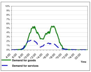
The progression of demand over the course of a day – measured as demand frequencies – according to Figure 1 shows a similar profile – but with different levels – for goods and for services with two maxima. Beginning at around 8 a.m. with increasing frequencies a first local maximum is achieved at 11 a.m.. Afterwards the frequency decreases until 2 p.m. and reaches the second local maximum at around 5 p.m.. Due to the limited opening hours 2001/2002 (workdays from 6 a.m. until 8 p.m. but with some exemptions) there is only a marginal demand at night between 8 p.m. and 7 a.m.
There are higher frequencies for the demand for goods than the demand for services throughout the day; the services’ maximum is earlier and relatively more pronounced in the morning.
Figure 1: Demand for goods and services 2001/2002 – total population (in percent)
0% 1% 2% 3% 4% 5% 6% 7% 8% 9% 10%
4:00 6:00 8:00 10:00 12: 00
14: 00
16:0 0
18:0 0
20:0 0
22: 00
24: 00
02: 00
Time
Demand for goods Demand for services
Source: German Time Budget Survey 2001/2002, own calculations
This global picture shows the expected demand peaks mornings and afternoons; however, an eventually expected higher demand frequency outside of the normal working hour (say after 5 p.m.) will not be visible in the picture of the total population.
Let us now ask for socio-economic group specific behaviour. Since any employment in principle restricts demand possibilities and thus has consequences on the individual consumption, we separate our single group specific analyses into the active population (Table 1 for aggregated time period and Figures 2-5 for the entire course of the day respectively) and the non-active population (Table 2 and Figures 2-5, too).
4.2 The Timing of Daily Demand – According to Gender
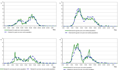
[image:10.595.141.455.292.542.2]for goods as well as for services the demand frequencies of the active population are consistently higher among women than among men. Less pronounced but more often, too, also non-active women buy relatively more often than non-active men: it’s the women who are the frequent buyers.
Active persons have two demand peaks, the morning at 11 a.m. and the afternoon at about 5 p.m. (the afternoon peak is more pronounced for goods than for services). The services’ peaks are earlier.
Figure 2: Demand for goods and services 2001/2002 – by sex and status of employment (in percent)
0 2 4 6 8 10 12 14
4:00 6:00 8:00 10:00 12:00 14:00 16:00 18:00 20:00 22:00 24:00 2:00 Tim e %
0 2 4 6 8 10 12 14
4:00 6:00 8:00 10:00 12:00 14:00 16:00 18:00 20:00 22:00 24:00 2:00
Tim e %
Demand for goods women (active population)
Demand for goods w omen (non-active population)
Demand for goods men (active population) Demand for goods men (non-active population)
0 1 2 3 4 5 6
4:00 6:00 8:00 10:00 12:00 14:00 16:00 18:00 20:00 22:00 24:00 2:00
Tim e %
0 1 2 3 4 5 6
4:00 6:00 8:00 10:00 12:00 14:00 16:00 18:00 20:00 22:00 24:00 2:00
Tim e %
Demand for services w omen (non-active population) Demand for services w omen (active population)
Demand for services men (non-active population) Demand for services men (active population)
Source: German Time Budget Survey 2001/2002, own calculations
Non-active women and men are more demand active than are active persons: they buy goods more frequent and request services more frequent. Non-active men and women make up the peak mornings.
Thus, gender specific differences with regard to the demand frequency over the day profile are proven in particular for the active population. A reason behind might be a gender difference in part-time and full-time occupation with different shopping possibilities.
4.3 The Timing of Daily Demand – According to Age Groups
[image:11.595.78.550.241.524.2]to show a different consumption pattern in general. The question here is whether these life cycle changes also involve an effect on the timing of daily demand behaviour.
Against the background of any employment overall there are no remarkable age effects on the timing of daily consumption: a similar timing pattern in all three selected age groups and connected phases of life with two peaks of demand frequencies at around ten to eleven and five o’clock (pronounced for goods in the afternoon; Figure 5) is given. As might be expected, older employed persons (50-64 years of age) compared to younger ones slightly more often ask for services.
Figure 3: Demand for goods and services 2001/2002 – by age groups and status of employment (in percent)
0 2 4 6 8 10 12 14
4:00 6:00 8:00 10:00 12:00 14:00 16:00 18:00 20:00 22:00 24:00 2:00 Tim e %
0 2 4 6 8 10 12 14
4:00 6:00 8:00 10:00 12:00 14:00 16:00 18:00 20:00 22:00 24:00 2:00
Tim e %
Demand for goods 15-29 (non-active popultaion) Demand for goods 15-29 (active popultaion) Demand for goods 30-49 (non-active popultaion) Demand for goods 30-49 (active popultaion) Demand for goods 50-64 (non-active popultaion) Demand for goods 50-64 (active popultaion)
0 1 2 3 4 5 6
4:00 6:00 8:00 10:00 12:00 14:00 16:00 18:00 20:00 22:00 24:00 2:00 Tim e %
0 1 2 3 4 5 6
4:00 6:00 8:00 10:00 12:00 14:00 16:00 18:00 20:00 22:00 24:00 2:00 Tim e %
Demand for services 15-29 (active popultaion) Demand for services 15-29 (non-active popultaion) Demand for services 30-49 (non-active popultaion) Demand for services 30-49 (active popultaion) Demand for services 50-64 (non-active popultaion)
Demand for services 50-64 (active popultaion)
Source: German Time Budget Survey 2001/2002, own calculations
For the non-active population, however, differences according to age appear: younger non-employed people (15-29 years of age) shop in the mornings and seek services in the afternoons. In contrast, the older non-active persons clearly prefer the mornings (for goods and service demand).
[image:12.595.85.548.259.541.2]4.4 The Timing of Daily Demand – According to the Economic Situation: Income Poverty
Income traditionally is the economic resource of demand and a central factor in microeconomic (neoclassical) consumption explanation. In addition, socio-economic factors of the consumers themselves and their environment are known and proven in many empirical studies. The question here is if the economic situation not only effects the level of spending but also the timing of daily demand behaviour; and in particular, if the consumption timing and/or frequency of persons from poor and non-poor households differ.
Active population: a similar demand timing profile appears between the „working poor“– active persons from poor households3 – with that of all other active persons (Figure 4). The timing profile of the demand for services of the „working poor“, however, is more irregular over the course of the day and less „smooth“ than that of the other active persons.
Figure 4: Demand for goods and services 2001/2002 – by income poverty and status of employment (in percent)
0 2 4 6 8 10 12 14
4:00 6:00 8:00 10:00 12:00 14:00 16:00 18:00 20:00 22:00 24:00 2:00 Tim e %
0 2 4 6 8 10 12 14
4:00 6:00 8:00 10:00 12:00 14:00 16:00 18:00 20:00 22:00 24:00 2:00 Tim e %
Demand for goods poor (active population) Demand for goods poor (non-active population) Demand for goods non poor (active population) Demand for goods non poor (non-active population)
0 1 2 3 4 5 6
4:00 6:00 8:00 10:00 12:00 14:00 16:00 18:00 20:00 22:00 24:00 2:00 Tim e %
0 1 2 3 4 5 6
4:00 6:00 8:00 10:00 12:00 14:00 16:00 18:00 20:00 22:00 24:00 2:00 Tim e %
Demand for services poor (non-active population) Demand for services poor (active population) Demand for services non poor (active population) Demand for services non poor (non-active population)
Source: German Time Budget Survey 2001/2002, own calculations
Non-active population: again, the timing profiles of the demand for goods and services of the poor and non-poor are similar in general but less “smooth” for the poor non-active.
Noticeable differences in the timing profiles in general are found again between the active and non-active population – no matter if poor or not poor: non-employed persons mainly
3
[image:13.595.75.549.325.607.2]prefer their demand in the morning while active persons prefer to shop and ask for services in the afternoon (with peak again around 5 o’clock).
The economic situation with emphasis on the poor all over shows no distinct different timing profiles, however, the timing profile of the poor is less “irregular”. With regard to income, thus, the working conditions have more or less the same effects to the "working poor" than to other active persons. A possible peripheral daily consumption because of low money income thus is not pronounced visible. A possible working time intensity and consequence of being poor because of low wages is another aspect which will be regarded in the following.
4.5 The Timing of Daily Demand – According to Daily Working Hour Arrangements
Working hour in general limit, at times prevent, the possibilities for shopping. A traditional full-time job obligating the person over the entire day is known to be receding, giving way to newer forms of daily working hour arrangements (key word: flexibility). The question here is whether different daily working hour arrangements which among others allow for intermissions with daily demand during working hour.
According to the timing and the fragmentation of the working day Merz and Burgert (2004) differentiated four daily working hour arrangements and showed that there are significant structural differences in the labour market accompanying this categorisation.
Timing of work in a day: Any description of working hour characteristics include information about the beginning, the duration and/or the end of the working hour. Here and in line with others we define the time between 7 a.m. and 5 p.m. as the core working hour.4 Therefore, there are two types of working days with respect to the timing of work: first, a working day in which the job is executed mainly during the core working hour, and second, a working day in which the work is performed mainly outside of the core working hour.
Fragmentation of a working day: A second dimension of a working day is its fragmentation. Fragmentation might be illustrated by the number of work intermissions. Then, it is possible to differentiate between a not fragmented work day, on the one hand, in which persons work in one „stretch“ and a fragmented work day, on the other hand, in which a person's work is interrupted by at least one „abnormal“ break. In order to not define short breaks (such as coffee breaks etc.) as important work intermissions, we assess breaks of more than one hour as important intermissions which allow some consumption time and/or a potential job change.
With the combination of both dimensions, timing and fragmentation, four basic working hour arrangements can be derived:
Category I (cat 1): not fragmented core working hour („normal“ working day) (65.2%)5
Category II (cat 2): fragmented core working hour (25.1%)
Category III (cat 3): not fragmented non-core working hour (6.4%)
4
In Germany most working days begin between 7am and 8am and end between 4 p.m. and 5 p.m.. This restriction on the core working hour complies with international studies (see e.g. Harvey et al, 2000).
5
Category IV (cat 4): fragmented non-core working hour (3.3%)
For 2001/2002 more than one third (34.8%) of the working days are „atypical“ if the continuous core working hour are still viewed as normal and typical.
As Merz, Burgert and Böhm (2008) have shown, these daily working hour arrangements not only form the basis for significant differences in the individual explanation of working hours, but also have significant and varying impacts on income.
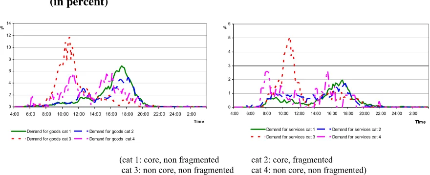
The question now is: do different working hour arrangements and thus a flexibility of the working conditions also have an impact on the daily demand? The answer: obviously (Figure 5) the demand for goods and services is influenced in different ways by the daily working hour schedules. The influence of the core working hour is as expected: if the core working hour are throughout the day („normal“ work day), the demand frequency moves to the evening (cat 1 and 2) and vice versa (cat 3 and 4). A fragmented work day, of course, allows for shopping during the course of the day; the respective category 2 and 4 confirm this. Noticeable is that active persons whose core working hour are after 5 p.m. and who have a fragmented work schedule (most atypical job), shop and demand services in the morning or before job starting in the afternoon. The shop opening hours of the survey year, not allowing late shopping certainly, is obviously limiting.
Figure 5: Demand for goods and services 2001/2002 – by working hour arrangements (in percent)
0 2 4 6 8 10 12 14
4:00 6:00 8:00 10:00 12:00 14:00 16:00 18:00 20:00 22:00 24:00 2:00 Tim e %
0 1 2 3 4 5 6
4:00 6:00 8:00 10:00 12:00 14:00 16:00 18:00 20:00 22:00 24:00 2:00
Tim e %
Demand for services cat 1 Demand for services cat 2 Demand for goods cat 1 Demand for goods cat 2
Demand for services cat 3 Demand for services cat 4 Demand for goods cat 3 Demand for goods cat 4
(cat 1: core, non fragmented cat 2: core, fragmented cat 3: non core, non fragmented cat 4: non core, non fragmented)
Source: German Time Budget Survey 2001/2002, own calculations
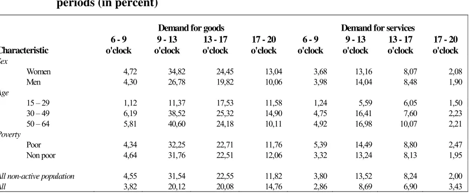
[image:15.595.80.520.379.558.2]Table 1: Demand for goods and services 2001/2002 of the active population in daily time periods (in percent)
Demand for goods Demand for services
Characteristic
6 - 9 o'clock
9 - 13 o'clock
13 - 17 o'clock
17 - 20 o'clock
6 - 9 o'clock
9 - 13 o'clock
13 - 17 o'clock
17 - 20 o'clock
Sex
Women 3,71 19,18 24,67 18,80 2,41 8,24 8,18 5,00
Men 3,21 9,84 13,98 14,32 2,33 4,40 4,57 3,52
Age
15 – 29 2,17 9,78 15,36 13,13 1,22 5,01 4,01 3,27
30 – 49 3,84 14,86 19,66 18,03 2,41 5,48 6,21 4,40
50 – 64 3,65 16,11 19,85 15,17 3,38 8,83 8,30 4,55
Poverty
Working poor 2,91 14,48 19,93 14,59 1,05 7,01 5,97 2,07
Working non poor 3,55 14,09 18,74 16,66 2,45 6,06 6,14 4,41
Working hour arrangements
cat 1 (not fragmented/core) 2,54 6,88 18,87 19,28 1,33 2,68 5,78 4,77 cat 2 (fragmented/core) 2,51 9,51 13,21 15,69 2,30 5,31 5,17 4,04 cat 3 (not fragmented/non-core) 5,63 32,77 8,80 4,61 1,79 12,67 2,92 1,27 cat 4 (fragmented/non-core) 6,80 15,26 16,03 6,32 3,69 4,32 4,78 0,85
All active population 3,43 14,02 18,76 16,32 2,36 6,12 6,19 4,18
All 3,82 20,12 20,08 14,76 2,86 8,69 6,90 3,43
Source: German Time Budget Survey 2001/2002, own calculations
Table 2: Demand for goods and services 2001/2002 of non-active persons in daily time periods (in percent)
Demand for goods Demand for services
Characteristic
6 - 9 o'clock
9 - 13 o'clock
13 - 17 o'clock
17 - 20 o'clock
6 - 9 o'clock
9 - 13 o'clock
13 - 17 o'clock
17 - 20 o'clock
Sex
Women 4,72 34,82 24,45 13,04 3,68 13,16 8,07 2,08 Men 4,30 26,78 19,82 10,06 3,98 14,04 8,48 1,90
Age
15 – 29 1,12 11,37 17,53 11,58 1,24 5,59 6,05 1,50 30 – 49 6,19 38,52 25,32 14,90 4,75 16,41 7,60 2,23 50 – 64 5,81 40,60 24,18 10,11 4,92 16,98 10,07 2,21
Poverty
Poor 4,34 32,25 22,71 11,76 5,39 14,49 8,80 2,47 Non poor 4,64 31,76 22,51 12,06 3,32 13,24 8,13 1,95
All non-active population 4,55 31,54 22,55 11,82 3,80 13,52 8,24 2,00
All 3,82 20,12 20,08 14,76 2,86 8,69 6,90 3,43
Source: German Time Budget Survey 2001/2002, own calculations
5
A Microeconomic Model for the Timing of Daily Demand for
Goods and Services
[image:16.595.75.540.415.608.2]life cycle (e.g. Hall 1998, Epstein and Zin 1989) quantifying the consumption substitution between life periods. The result of the static and intertemporal microeconomic modelling first of all is a set of demand equations explaining the optimal quantities/expenditures/activity durations by its (shadow) prices and income.
Our question about the timing of demand, however, focus rather on “when” (and not on the quantity of how long) within a time period a certain demand activity is done and seeks for explanation by socio-economic factors. In principle, the mentioned neoclassical intertemporal approach could be the microeconomic model for our timing focus. However, the more compact daily view and its activity time interdependencies ask for a more specific approach. We argue, in particular, that the interdependencies between single time periods of a day should be quantified by a simultaneous equation approach allowing period specific socio-economic explanation under interdependency rather than by an explicit more general time preference equation of the intertemporal neoclassical approach.
With the question “what drives to do shopping and the demand for services at a distinct time within a day” we face a typical discrete choice problem. Analogous to a complete demand system under the quantity perspective, we face something like a complete demand period system in the sense, that goods and services can be demanded by one person more than one time a day. So we face possible simultaneous demand in the morning and/or in the afternoon etc.
Considering this simultaneousness and based on a microeconomic utility maximisation approach, a rational decider will maximise his overall utility with regard to the utilities out of the choices to be active in one or more demand periods a day (t=1,...,T).
(1a) * * * * * * ,
1 1
( , ,..., , ) max!
i i ig is igT isT
u =u u u u u =
assuming a latent utility index * with demand period related stochastic utility indices
i
u
(1b) ,
* '
* '
( 1,..., )
igt gt i ijt ist st i ijt
u x
u x t
β ε
β ε
= +
= + = T
for the demand of any goods (index g) and for the demand for any services (index s) with xi
as a vector of socio-economic variables of the individual i (for example age, gender, income).
βgt and βst are the two parameter vectors for goods and services to be estimated for each
demand period t=1,…,T. The residuals εit will capture the interdependencies by multivariate
distributed error terms. Without loss of generality the set of explanatory variables xi might be
different for goods and for services.
A demand period related activity then is observed if the respective latent utility index exceeds a threshold with
(2) .
* '
*
1 0 . ,
0 0 1,...,
ijt jt i ijt ijt
ijt
if u resp x j g s y
if u t T
β ε
⎧ > > =
⎪ = ⎨ ≤ = ⎪⎩ 6 6
The symmetry of the assumed normal distribution allows the specification β ' <ε
jtxi ijt instead of
'
The error terms εijt over all demand periods a day will be multivariate normally distributed with a respective expected value of zero (E(εijt)=0) and a variance-covariance matrix V, with ones on the main diagonal and otherwise the correlations ρtk =ρkt ( ,t k=1,..., ,T t ≠k) . The demand probability in one demand period a day then is
(3) Pjt
(
yijt = =1)
Pjt(
uijt* >0)
=Pjt(
εijt <βjt' xi)
= Φ2T(βjt' xi)
with as a 2*T-dimensional standard normal distribution. This demand probability is at the core of the following analysis.
2 (.)
Φ T
One might argue that the timing of shopping does not spend direct utility as comparable to actually buying and consume something. However, restricted by time in general, a decision finally has to be done, when shopping will happen. So, there is a typical discrete choice problem with some underlying and latent individual utility tackle which finally – by exceeding a critical level – yields the observable decision to shop or demand for services within a certain period a day.
6
Multivariate Explanation of the Timing of Daily Demand for
Goods and Services
Following our microeconomic model for the timing of daily demand for goods and services (equations 1-3) we estimate the demand probabilities for demand periods a day by a Multivariate/Simultaneous Probit Model (MPV)7. As it is well known, a respective Maximum Likelihood estimation based on a multidimensional normal distribution is very expensive with regard to the non-analytical solution of the multidimensional normal integral. We have used the Stata procedure (“multivariate probit regression”) from Capellari and Jenkins (2003) which follows the Geweke-Hajivassiliou-Keane (GHK) approach for a simulation estimator. The GHK simulator has advantageous characteristics: the estimated coefficients are unbiased, the simulated probabilities lie in the interval (0;1) and are a continuous and differentiable function of the model parameter (Börsch-Supan and Hajivassiliou (1993)). In addition to the respected correlation over equations we have to deal with expected correlation over observations with our data. Since each person delivers two respective three days with diary data we face clustered data where the error terms are expected not to be distributed independently of the observations. To achieve consistent estimates we therefore use robust White variance estimates accounting for clustering.8
The following estimation of the probabilities of the timing of daily demand for goods and services – as with our descriptive analysis – will consider simultaneously four (T=4) demand periods a day: early (6a.m.-9a.m.), mornings (9 a.m.to 1 p.m.=13 o’clock), afternoons (1 p.m.-5 p.m.=17 o’clock) and evenings (p.m.-5 p.m.-8 p.m.=20 o’clock) ((t=1,...,T with T=4). These definitions follow typical opening hours in Germany at the survey time 2001/2002. If there is
7
In the literature, discrete choice models use the term “multivariate” in a simultaneous sense though “mutivariate” often refers only to multiple influencing factors.
8
more than one consumption activity in one of our three hour demand periods a day then they are considered as a single combined demand activity. As the descriptive results has shown the timing of the demand for goods is different than the timing of the demand for services. So we will have four different equations for goods and four different equations for services, which, however, are allowed to be correlated each other within the simultaneous eight equation system.
The choice of the explanatory variables, and thus the hypotheses about socio-economic influences to be tested, are based on hypotheses of theoretical and empirical consumer and labour economics (see Blackwell et al. 2001, Blundell et al. 1993) and results of our descriptive analyses. As mentioned, microeconomic consumer theory relies on prices for goods and on income when explaining optimal allocated consumption quantities. With our cross-sectional data prices are not available; income as an important explanatory factor in consumer goods’ quantity analyses, however, will be tested here for the timing of demand. In addition, the explanation will be extended by the following set of individual socio-economic variables with personal, household and regional characteristics.
Personal set: we test personal characteristics (like gender, age as a proxy for the life cycle situation), human capital variables roughly describing all day management skills, time spent for non-market activities (as competing in time allocation) at the observed day and working conditions for persons in the labour market9 (like being self-employed with an expected time sovereignty, personal monthly net income, commuting time and daily working hour arrangements with timing and fragmentation work characteristics).
Household/family set: we test the partner’s employment influence (like the partner’s full or part-time hours of work), household characteristics (like household size and children) and the economic situation of the household to be poor or not as well as the household residual income (without the individual personal income under investigation) as a proxy for the available household wealth;
Regional set: we are able to test the still expected general different living conditions and shopping/demand possibilities between West and East Germany.
Local demand: we test whether shopping and services possibilities within walking distances are influencing.
Since it has already been shown in the descriptive analysis that any employment has an explicit effect on the timing of demand for goods and services, separate estimations for the active and non-active population will be carried out.10 Both estimations therefore will differ with respect to the employment situation in particular. Because of this we only include persons at the working age between 15 and 64 years old. We concentrate on the work week (Monday to Friday) because the demand behaviour on the weekends differs considerably from that of the work week.
9
With competing non-market and paid working time as exogeneous, independent x-variables we assume that demand activities are the result of these non-market and paid working allowing to buy goods and services. This might be a problem when the duration of demand would be analyzed (concurrent time allocation) but will be of minor importance by our analysis of the timing of demand.
10
6.1 Goodness of Fit and the Importance of Simultaneous Over-the day Demand
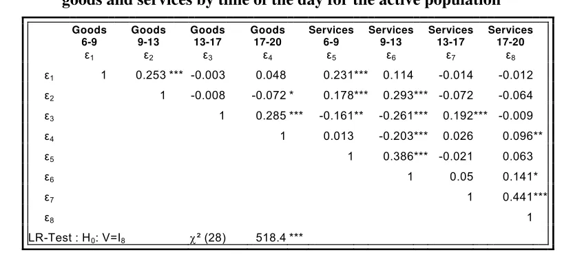
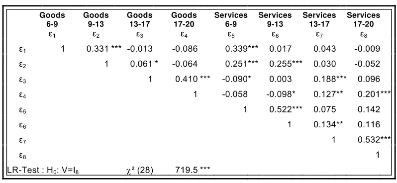
[image:20.595.86.494.291.476.2]The timing of the daily demand (as a further used shortcut for the probability of the timing of daily demand for goods respective services) overall is significantly explained by our model, not only for the active population but also for the non-active population (Likelihood Ratio test with = 0.1%); see Tables 3 and 4. The final correlation matrix of the error terms for the Multivariate Probit estimation for the active population in Table 3 and the non-active population in Table 4 is organized in a goods’ and services’ block structure for its four time periods. Early and morning shopping as well as afternoon and evening shopping is highly correlated showing overlapping demand activities. This is true also for the demand for services. The interdependence between shopping for goods and asking for services is strong for each daily period (highly significant positive correlation).
Table 3: Correlation Matrix for the Multivariate Probit estimation of the demand for goods and services by time of the day for the active population
Goods 6-9
ε1
Goods 9-13
ε2
Goods 13-17
ε3
Goods 17-20
ε4
Services 6-9
ε5
Services 9-13
ε6
Services 13-17
ε7
Services 17-20
ε8
ε1 1 0.253 *** -0.003 0.048 0.231*** 0.114 -0.014 -0.012
ε2 1 -0.008 -0.072 * 0.178*** 0.293*** -0.072 -0.064
ε3 1 0.285 *** -0.161** -0.261*** 0.192*** -0.009
ε4 1 0.013 -0.203*** 0.026 0.096**
ε5 1 0.386*** -0.021 0.063
ε6 1 0.05 0.141*
ε7 1 0.441***
ε8 1
LR-Test : H0: V=I8 χ² (28) 518.4 ***
* p-value<0,05 / ** p-value<0,01 / *** p-value<0,00 Source: German Time Budget Survey 2001/2002, own calculations
Table 4: Correlation Matrix for the Multivariate Probit estimation of the demand for goods and services by time of the day for the non-active population
Goods 6-9
ε1
Goods 9-13
ε2
Goods 13-17
ε3
Goods 17-20
ε4
Services 6-9
ε5
Services 9-13
ε6
Services 13-17
ε7
Services 17-20
ε8 ε1 1 0.331 *** -0.013 -0.086 0.339*** 0.017 0.043 -0.009 ε2 1 0.061 * -0.064 0.251*** 0.255*** 0.030 -0.052 ε3 1 0.410 *** -0.090* 0.003 0.188*** 0.096 ε4 1 -0.058 -0.098* 0.127** 0.201***
ε5 1 0.522*** 0.075 0.142
ε6 1 0.134** 0.116
ε7 1 0.532***
ε8 1
LR-Test : H0: V=I8 χ² (28) 719.5 ***
* p-value<0,05 / ** p-value<0,01 / *** p-value<0,00 Source: German Time Budget Survey 2001/2002, own calculations
Though we face two prominent daily demand regimes we will see that the single significant results and differences of the demand period specification support the prominent importance of the chosen four daily demand period thresholds.
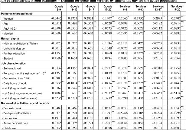
6.2 Microeconometric Results of the Probabilities for the Timing of Daily Demand – Active Population
6.2.1 Daily Demand for Goods – Active Population
Let us start with the consumption situation, the demand for goods, of the active population. Which hypotheses then are of particular meaning for the probability to shop in a certain daily demand period? Table 5 shows the results. Out of the set of personal characteristics gender and age show a significant influence for all demand periods from 9 o’clock on but in different magnitudes.11 12 The significant shopping probability of women – with the exemption of early in the morning – is always greater than that of men. Age, as a course of life indicator, is a significant predictor with non-linear importance in particular in the afternoon and in the evening. The combined non-linear age influence shows an increasing probability effect until 46 to 48 years (and then decreasing) for the morning and afternoon/evening shopping. The family status to be married neither restricts nor fosters shopping in any demand period. Interestingly, a hypothesis of human capital influences via expected management skills cannot be confirmed.
11
The underlying descriptive statistics of the database for estimation can be found in the Appendix Table 14.
12
Table 5: Mulitvariate Probit Estimates – Demand for goods and services by time of the day for the active population
Goods 6-9
Goods 9-13
Goods 13-17
Goods 17-20
Services 6-9
Services 9-13
Services 13-17
Services 17-20
Personalcharacteristics
- Woman -0.0445 0.2727*** 0.2831*** 0.1407** 0.2065* 0.1755* 0.2995*** 0.2407***
- Age 0.0511 0.0497** 0.0553*** 0.0629*** 0.0398 0.0070 0.0192 0.0814***
- Age² 10-2 -0.0509 -0.0510* -0.0587*** -0.0673*** -0.0425 0.0028 -0.0112 -0.0897***
- Married -0.0698 -0.0635 -0.0602 -0.0589 -0.2895 -0.2877* -0.0622 -0.0282
Humancapital
- High school diploma (Abitur) -0.0070 0.0775 0.0096 0.1084* -0.1311 -0.0425 -0.0255 -0.0733
- University degree 0.0013 -0.0018 0.0655 -0.1549* -0.0325 -0.0226 -0.0634 0.0818
- Further education -0.1153 0.0220 0.0310 0.0260 0.0119 0.1376* 0.0200 0.0238
- Student 0.4597* 0.1654 -0.1656 0.0494 0.0803 -0.0957 0.2135 -0.2364
Jobcharacteristics
- Self-employed 0.0137 -0.1353 -0.2871*** -0.2972*** 0.3672** 0.2928** -0.0310 -0.1759
- Personal monthly net income * 10-3 -0.1350* 0.0168 0.0108 0.0179 0.1512*** 0.0451 0.0737* 0.0253
- Commuting time * 10-2 0.0983 -0.0770 -0.3878*** 0.1141 0.1607 0.0972 -0.3035* -0.0218
- Daily hours of work -0.0536** -0.1014*** -0.1261*** -0.0414*** -0.1071*** -0.1375*** -0.1441*** -0.0443**
- cat 2 (fragmented/core) 0.0162 0.2547*** -0.1418** -0.1031* 0.2563** 0.3108*** -0.0625 -0.0387
- cat 3 (not fragmented/non-core) 0.4082** 1.0676*** -0.8740*** -0.9079*** 0.3467* 0.7416*** -0.6453*** -0.5114**
- cat 4 (fragmented/non-core) 0.6236*** 0.5711*** -0.1730 -0.3739** 0.2590 0.3436 -0.3193 -3.7706***
Non-market activities/ social network
- Domestic work 0.0489 0.0469* -0.0024 -0.0672*** -0.0353 -0.0085 -0.0405 -0.1349***
- Do-it-yourself activities -0.0370 -0.0221 -0.0807 -0.1297** -0.5966 -0.1105 -0.0224 -0.1998*
- Home care 0.1913 -0.0441 0.1190 0.0117 -1.0352 -0.1557 -0.1255 -0.1099
- Active personal help 0.0145 -0.0395 -0.0771 -0.2257*** -0.0064 -0.0450 -0.1124 -0.1911
Table 5 (cont.)
Goods 6-9
Goods 9-13
Goods 13-17
Goods 17-20
Services 6-9
Services 9-13
Services 13-17
Services 17-20 Partner’s employment status
- Full time 0.0270 0.1764* 0.2100** 0.1456* 0.1610 0.2093 0.0821 -0.0881
- Part time -0.3513** 0.0597 -0.0048 0.0350 0.2046 0.2161 0.1978* 0.0177
- No partner -0.0787 0.0822 0.0836 0.1200 0.1069 0.0519 0.1158 0.1258
Household characteristics
- Hh-size 0.0320 -0.0522 -0.0577* -0.0573* 0.0060 0.0411 0.0076 -0.0185
- Hh with children -0.0786 0.0680 0.1737** 0.0651 -0.0135 -0.1046 -0.0308 0.0115
- Hh under poverty line -0.4406* -0.2873 0.0171 0.1151 -0.4495 -0.3773 0.0566 -0.2440
- Hh residual net income 10-3 -0.0437 0.0068 -0.0186 0.0063 0.0347 -0.0220 0.0078 0.0008
Region
- East germany -0.1495 0.0247 0.0907 0.1768*** 0.2637** 0.0562 0.0942 0.2810***
Local possibilities for…
- shopping -0.2456 -0.1451 0.1220 0.1070 0.2231 0.0469 0.1928 0.0338
- service demand 0.1572 -0.0807 -0.0787 -0.0163 0.0487 -0.0054 0.0522 -0.0753
Constant -2.3187*** -1.9368*** -1.2224*** -2.0056*** -2.9418*** -1.6415*** -1.6029*** -3.0372***
Wald - χ² (240) 5427.7***
Log pseudolikelihood -13244.5
n 7079
[image:23.792.67.696.104.440.2]As to our hypothesis, the dominance of a working day will influence the timing of shopping. The hypothesis that a self-employment with a higher degree of time sovereignty than being an employee prefers a “within the day shopping” is only indirectly confirmed: a self-employment significantly reduce the probability of an afternoon and evening shopping. Daily working hour arrangements with its timing and fragmentation overall have significant impacts on the timing of shopping goods. In comparison to the reference category cat I (core working hour throughout the day), all other categories increase the demand probability until noon and decrease it afterwards with categorical-specific differences. Thus a fragmented work day and non-core working, as expected, enable shopping over the day accordingly.
There is one astonishing result according the economic situation: neither the personal monthly net income nor the available further income resources of the household have a significant influence on the shopping probability in the demand periods of a day. The minor exemptions: significantly (α=5%) less early shopping for all workers and significantly (α=5%) less morning shopping hours for the poor, here the "working poor". Thus, consumer theory based income influence might be a driving factor for consumption expenditures respective consumption quantities, however, income is not prominent and distinctive for the probability to shop in neither daily demand period, a remarkable result.
Household/family situation: the timing of daily shopping seems to be independent from
competing hours spent in non-market activities like child care and nursing other household members. Domestic work is in favour for shopping in the morning for the burden of the evening. Active personal help in social networks will be done in the afternoon and diminishes the respective shopping probability significantly. The partner’s full time employment has significant impacts on the shopping timing in the afternoon and in the evening. Together with the working day situation of the person under investigation partner shopping will be visible later the day. Further household characteristics as the size, a household with children, and the economic situation of the household including being poor are not significant.
Regional differences in the timing of daily shopping between West and East Germany are
only significant in the evenings with significant greater evening shopping probabilities living in East Germany. It would be interesting what will be behind; the data here only allows speculation.
Local demand possibilities: The hypothesis, that the timing of shopping is influenced by nearby local shopping possibilities cannot be confirmed.
6.2.2 Daily Demand for Services – Active Population
As we have already seen in the description, the daily service demand differs from the goods’ demand in its frequency level and over the day profile. In contrast to the demand for goods, it is noticeable that gender only has a significant impact with active persons; non-active women and men show a similar timing of the demand for services (see Table 6). Probably due to working hour restrictions economically active older persons increasingly (until 45 years) ask for services in the evenings. To be married or not is not significant for the demand for services probably because of husband independence of genuine personal belongings.
reference to the timing and fragmentation are also notably decisive for the timing of the daily demand for services.
The economic situation and main microeconomic demand resource – personal income as well as the household residual income – had surprisingly no effects on the timing of shopping hours (with the early exemption of personal income of active persons, α=5%). Here again, neither personal nor household income effect the timing of daily demand for services (with the early exemption of personal income of active persons, α=0,1%). Similar to restrictions of a paid work, unpaid work in a household or personal help for others is restricting and do significantly influence the timing of the daily demand for services.
So, domestic work or do-it-yourself reduce the evening demand for active and non-active population. Also an engagement in social networks by helping others will reduce the probability of evening demand for services. In addition, the assumption, that services are often person-associated and therefore not transferable, is supported by the finding that the partner’s employment as well as the further household situation, show no significant influence on the daily demand for services. As with the demand for goods, some regional influences on the timing of daily demand for services can be observed: in East Germany the respective probability after core working hour (before 9 a.m. and after 5 p.m.) is greater than in West Germany (workers).
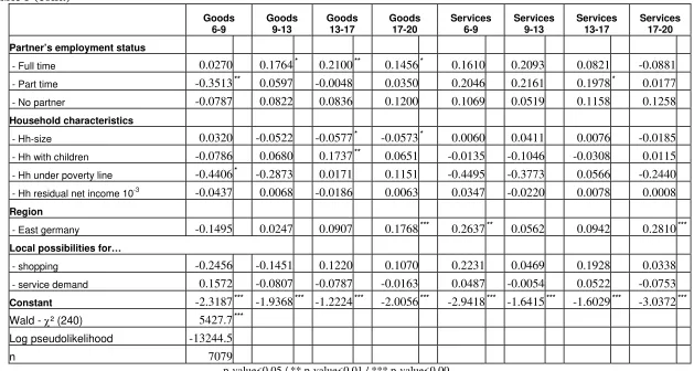
6.3 Microeconometric Results of the Probabilities for the Timing of Daily Demand – Non-Active Population
6.3.1 Daily Demand for Goods – Non-Active Population
Microeconometric results for the probability for the timing of daily demand for the non-active population are shown in Table 6. Personal characteristics as gender and age (non-linear) again are significant in explaining the demand probabilities in all daily demand periods for persons not in the labour force. Non-active women prefer to go shopping in the afternoon. For all periods a day the increasing non-linear age influence is significant and in favour for the respective period in the day. However, the respective year when the influence starts to decrease is different for each period: early 53 years, morning 57 years, afternoon 51 years and evening 44 years. Thus the influence of the elderly in the afternoon and evening is less pronounced than early and mornings.
Similar to the active population, human capital variables do not influence significantly the timing of goods’ demand. In some contrast to the active persons, however, non-market activities and an engagement in social networks have different impacts on the timing of shopping over the day: those activities can be and are done without paid working restrictions within a full day and thus influence the shopping probabilities significantly over the day. Children will rise the probability of morning shopping probably because of being in school in the morning. The partner’s employment status and all further household characteristics
Table 6: Mulitvariate Probit – Demand for goods and services by time of day for the non-active population
Goods 6-9
Goods 9-13
Goods 13-17
Goods 17-20
Services 6-9
Services 9-13
Services 13-17
Services 17-20
Personalcharacteristics
- Woman -0.0827 0.1435** 0.2259*** 0.1661** -0.0318 -0.0004 0.0676 0.0990
- Age 0.0912*** 0.0935*** 0.0571*** 0.0516*** 0.0809*** 0.0964*** 0.0378** 0.0512**
- Age² 10-2 -0.0859*** -0.0815*** -0.0560*** -0.0581*** -0.0782*** -0.0946*** -0.0312 -0.0591*
- Married -0.1829 0.1858 0.0981 -0.0991 0.1705 0.0451 0.1957 -0.0615
Humancapital
- High school diploma (Abitur) 0.0332 0.1403 0.1242 0.1669 0.0653 0.1984* 0.0629 0.1129
- University degree 0.1848 -0.0308 0.1164 -0.0797 0.3233* -0.1165 -0.1608 -0.0475
- Further education -0.1233 -0.0108 0.0128 0.0533 0.0798 -0.0209 -0.0035 0.1348
- Student 0.1910 -0.0490 0.0268 0.0036 -0.2051 -0.2154 -0.1469 -0.1843
Non-market activities/ social network
- Domestic work 0.0048 -0.0124 -0.0412*** -0.0459*** -0.0204 -0.0960*** -0.0495*** -0.0549**
- Do-it-yourself activities -0.0316 -0.0870* -0.0765* -0.0102 -0.1046 -0.1330* -0.0442 0.0649
- Home care -0.2311 -0.0396 -0.1165 0.0098 -0.1289 0.0250 -0.0614 -0.7180
- Active personal help 0.0315 -0.0765*** -0.0834*** -0.0817* -0.0902 -0.1467*** -0.1116** -0.0418
Table 6 cont.
Goods 6-9
Goods 9-13
Goods 13-17
Goods 17-20
Services 6-9
Services 9-13
Services 13-17
Services 17-20
Partner’s employment status
- Full time 0.1928 0.0809 -0.0372 0.2189** 0.1456 0.1198 0.0355 0.1336
- Part time 0.0574 -0.0829 -0.1014 0.1014 0.0968 -0.0370 -0.0189 -0.0099
- No partner -0.2134 0.0984 0.1379 0.0739 0.2706 0.0072 0.3910* 0.1834
Household characteristics
- Hh-size 0.0424 -0.0080 -0.0020 0.0027 -0.0777 -0.1378*** -0.0239 0.0298
- Hh with children -0.0602 0.0598 0.0978 0.0435 0.2207 0.0937 0.0552 -0.0770
- Hh under poverty line 0.1190 0.0516 -0.0358 -0.1023 0.0907 0.0348 -0.0617 -0.1842
- Hh residual net income 10-3 0.0267 -0.0077 -0.0154 -0.0206 -0.0307 0.0010 -0.0198 -0.0836*
Region
- East germany 0.1733* 0.0983 0.0367 -0.0976 0.3269*** 0.1197 0.0614 0.1293
Local possibilities for…
- shopping -0.0795 0.1565 0.1230 -0.0624 0.1351 0.0922 0.0958 -0.2164
- service demand 0.0504 0.0970 -0.0571 0.1554 -0.0489 0.0537 -0.0026 0.2178
Constant -3.9027*** -3.3185*** -2.2245*** -2.2544*** -3.8132*** -2.9023*** -2.5067*** -2.8040***
Wald - χ² (184) 1210.2***
Log pseudolikelihood -11273.6
n 4743
6.3.2 Daily Demand for Services – Non-Active Population
Gender does not influence the timing for the demand for services in all periods of a day. Age again is important and is different in explaining the time when services are asked. The years when the non-linear age effect starts to decrease is about 50 years in the morning but 43 years in the evening which is in favour for morning services. Non-market activities like domestic work or active personal help for others decrease the demand for services in the mornings and evenings in some favour for early and late voluntary support of other persons. Some morning restrictions are visible: a larger households asks for morning activities which reduce the demand for services. Furthermore, early demand for services in East Germany is more probable among non-active persons. Here it can be speculated that a former long-term high employment rate of the population and generally other working hour conditions in East Germany would lead to a higher demand for services at the edges of a day. Local availability of services has no influence again in all periods of a day.
6.4 Some general conclusions
The simultaneous modelling and estimation has proven as to be necessary and important for the active as well as for the non-active population in explaining its different timing of daily demand for goods and services. The single results have shown that the timing decision differently depend on socio-economic respective socio-demographic factors.
What is the general picture behind all these single influences? Any paid employment indeed has impacts mainly via its timing restrictions on the daily shopping hours for goods and the demand for services. Also by the results of the non-active population, there are indirect impacts of available time from diverse non-market and social network unpaid work and activities for the timing demand pattern. In contrast to consumer theory and many empirical studies on consumption expenditure, neither the personal income nor the household’s residual income as the economic resource for consumption show significant influence on the timing of demand for goods and services; a remarkable result both for the active and the non-active population. There are significant regional differences with increased demand probabilities for goods and services early or late a day in East Germany. However, human capital, the family status and further household characteristics do not have an overall significant influence with regard to the demand for goods and services; once again a remarkable result for the active and the non-active population. It is rather gender, the course of life, time spent in paid market and/or own non-market activities, the partner’s situation and some regional aspects which differently influence the timing of daily demand for goods and services