The Price Marginal Cost Markup and its Determinants in U S Manufacturing

Munich Personal RePEc Archive

The Price-Marginal Cost Markup and its

Determinants in U.S. Manufacturing

Mazumder, Sandeep

Wake Forest University

September 2009

The Price-Marginal Cost Markup and its

Determinants in U.S. Manufacturing

Sandeep Mazumder∗

September 2009

Abstract

This paper estimates the price-marginal cost markup for US manufacturing using

a new methodology. Most existing techniques of estimating the markup are a variant

on Hall’s (1988) framework involving the manipulation of the Solow Residual. However

this paper argues that this notion is based on the unreasonable assumption that labor

can be costlessly adjusted at a fixed wage rate. By relaxing this assumption, we are

able to derive a generalized markup index, which when estimated using manufacturing

data is highly countercyclical and decreasing in trend since the 1960s. When we then

seek to explain what causes the manufacturing markup to behave in this way, the most important determinant is the share of imported goods in the industry. Thus, increasing

foreign competition in manufacturing has led to a decline in the industry’s markup over

time.

JELClassification: D24, D40, E32

Keywords: Markup; Marginal Cost.

∗_{Address: Sandeep Mazumder - Wake Forest University - Department of Economics - Carswell Hall - Box}

1

Introduction

The markup of price over marginal cost is an important concept in both industrial orga-nization and macroeconomics due to the implications it has for market competition, and for determining the extent to which excess capacity exists in an industry. However, since marginal cost is not directly observable, the markup is not straightforward to estimate from data. Therefore careful thought is required as to how we should first measure marginal cost, which then allows us to produce an estimate of the markup.

For many years, the markup was computed using an approach that focused on estimating the slope of the demand schedule (for a survey of this work see Bresnahan (1989)). However, Hall’s (1986, 1988) methodology then displaced this as the most popular framework, which remains as the foundation of the majority of papers that are written even today. Hall empha-sizes the significance of imperfect competition if we are to understand cyclical fluctuations, and he does this by manipulating the Solow residual equation to include a markup of price over marginal cost, based on the assumption of constant returns to scale. Essentially, Hall’s framework tries to estimate marginal cost as the observed change in cost as output changes from one year to the next. This methodology is then applied to US manufacturing data, which allows Hall to derive estimates of the markup.

Many papers have since been written which also estimate the markup, most of which are based on Hall’s (1988) methodology, or often some extension of it. For example, Eden and Griliches (1993) and Galeotti and Schiantarelli (1991) examine markups over marginal cost by modifying the production function that is used, while Shapiro (1987) starts with Hall’s work1_{, but then builds on this by suggesting new ways in which to estimate the market}

elasticity of demand. Domowitz, Hubbard, and Petersen (1988) also extend Hall’s analysis by including intermediate inputs (materials), and by allowing the markup to vary over time. Since Hall (1988) is of critical importance to how markups are estimated in macroeco-nomics and industrial organization literatures, we would like this approach to be the closest approximation to reality that we can achieve. However, closer examination of the method-ology exposes that same problem as Mazumder (2009) finds when examining how authors measure marginal cost. That is, Hall’s (1988) method is based on the implicit assumption

1

that labor can be freely adjusted at a fixed wage rate. Since we can think of labor being the product of the number of employees and the number of hours that they work, Hall’s implicit assumption requires that employment and/or hours can also be freely adjusted a fixed real wage rate. However Mazumder (2009) points out that employment is quasi-fixed due to adjustment costs that exist, and varying hours often requires varying the wage rate as well. Hence labor cannot be flexibly adjusted at a fixed wage rate. Indeed, Hall’s approach becomes even more problematic when we start to think about adjustment costs of capital, which are also ignored in that particular setup.

This paper proposes a solution to this problem by extending the work from Mazumder (2009). In this paper, a new measure of marginal cost is developed which accounts for the existence of adjustment costs of labor. This idea is based on Bils (1987) which states that we can measure marginal cost along any margin, holding all other inputs fixed at their optimal levels, assuming that firms optimally minimize costs. In particular, I choose to vary employees’ hours of work, while also recognizing that overtime pay exists in industries that are paid an hourly wage rate. This approach is then applied to manufacturing data, which yields a new measure of marginal cost. Given this new method of estimating marginal cost, it is then straightforward to compute a markup ‘index’ for the manufacturing sector, which can also then be re-estimated at further disaggregated levels. This measure is in index form due to data limitations on price levels, which means that we do not learn about the absolute levels of the markup, but rather we have information about the change in its trend over time and its movement over the business cycle.

paper therefore obtains a new measure of the markup which exhibits a considerable downward trend over time and moves counter to the business cycle, and one can argue that the method used is simpler than previous techniques, and based on more reasonable assumptions.

Given this new measure, this paper then seeks to explore what the determinants of the markup are, in a similar theme to Domowitz, Hubbard, and Petersen (1988). Specifically, this paper considers what role business cycles, domestic competition, foreign competition, and oil prices play in the movement of the manufacturing markup, using a time series framework–

something which has not been done before in the literature. The model is estimated by a two-stage dynamic OLS procedure to account for cointegrated variables, in a similar theme to Lettau and Ludvigson (2001). The results suggest that foreign competition–as measured by the share of manufactured goods that are imported–is the main determinant for the decline in the manufacturing markup, which can be most noticeably seen in the durables sector. Domestic competition has also played an important role, although to a much lesser extent than foreign competition. Therefore this paper finds that the increasing share of goods that are imported is the main determinant behind the decline in manufacturing’s markup, which is in keeping with the popular belief that competition from overseas has strongly affected this industry.

2

Existing Markup Methodology

Before developing a new markup index, it is important to critically examine the existing methodology that is prevalent in the literature, founded on the work of Hall (1988). In his paper, Hall uses the common definition for the markup ratio of: 𝜇 =𝑃/𝑋ˆ, where 𝑃 is the price level and 𝑋ˆ is nominal marginal cost. Therefore, to estimate the markup one needs a specification of marginal cost, which Hall specifies as:

ˆ

𝑋= 𝑊Δ𝐿+𝑅Δ𝐾

Δ𝑌 −𝜃𝑌 (1)

to output by the amount in which output would have risen in the absence of more capital or labor, where𝜃 is the rate of Hicks-neutral technical progress2_{. The numerator is the change}

in costs, where the cost function is given by 𝑊 𝐿+𝑅𝐾, and changing output by one unit induces a change in labor (Δ𝐿) and a change in the capital stock (Δ𝐾). The denominator is the change in output, adjusted for technical progress. The rationale for this specification of marginal cost is that we can compute marginal cost by looking at the changes of the inputs of production, namely𝐿 and 𝐾, while assuming that these factors are paid a fixed price of

𝑊 and 𝑅.

However if we reconsider equation (??), a significant limitation emerges. That is, by writing marginal cost in this way we are ignoring any adjustment costs to labor and capital. More specifically, (??) assumes that labor can be freely adjusted at a fixed wage rate, 𝑊. However, as Mazumder (2009) argues at length, labor input should really be thought of as the number of employees (𝑁) multiplied by the average number of hours each of them works (𝐻) such that 𝐿 = 𝑁 𝐻, and the evidence is that neither 𝑁 nor 𝐻 can be freely adjusted at a fixed wage rate. As Oi (1962) argued in his seminal paper, employment has adjustment costs such as recruitment and training costs, which means that𝑁 cannot be easily changed without incurring some other cost that is not captured by𝑊Δ𝐿. On the other hand, while the consensus is that 𝐻 can be flexibly varied with little-to-no adjustment costs, we know that adjusting hours often requires overtime pay, particularly in industries that are paid an hourly wage rate. Many labor economists, such as Lewis (1969), have explored this idea and concluded that the existence of overtime pay means that the wage rate cannot be fixed, but must instead be a function of hours,𝑊(𝐻). Therefore, the change in costs that is due to a change in labor is inaccurate when written as𝑊Δ𝐿, not to mention the large literature that deals with the adjustment costs of capital,𝐾. This paper then seeks to estimate the markup, based on a measure of marginal cost that does account for the existence of adjustment costs. In terms of the econometric implementation of Hall’s idea, there are also problems of selecting adequate instruments for𝜃𝑡 (for example, see Roeger (1995)) and many others also

argue that it is undesirable to assume constant returns to scale. Indeed, constant returns to scale implies that (??) is actually equivalent to average cost (see Hylleberg and Joergensen

2

(1998)), which is problematic in the event of phenomena such as overtime premia or adjust-ment costs. In addition, much of the literature also tries to compute 𝜇 using annual data, which in itself is questionable since we expect marginal cost to exhibit far greater short-run volatility within a year rather than at the annual frequency.

It must also be noted that alternative methodologies also exist, such as Rotemberg and Woodford (1990) who compute markups by looking at firms’ profit maximizing labor demand with an imperfectly competitive market structure. Their methodology does incorporate the notion of overhead labor requirements, but it requires assigning numerical values to the steady-state markup, to the elasticity of substitution between capital and labor, and it also assumes that wages and technology have the same trend growth rates. These things are not ideal when it comes to estimating the markup in a relatively simple way.

Overall there are several features to the existing methodologies of estimating the markup that are quite limited, and the literature would benefit from a simpler method that is based on more reasonable assumptions.

3

Nominal Marginal Cost

3.1 Estimation Methodology

In order to estimate marginal cost in a way that acknowledges the existence of adjustment costs to labor, this paper implements the idea set forth by Bils (1987)–that we can measure marginal cost by examining the cost of changing output along any one margin while holding all other inputs fixed at their optimal levels. While other methods that try to improve upon the measurement of marginal cost exist–see Rotemberg and Woodford (1999) for a selection of these approaches–this paper chooses to focus on one particular generalization that is simple and easy to implement. Yet this method is powerful in the sense that it allows us to derive a new estimate of marginal cost that accounts for adjustment costs of labor.

notation, we can then express Bils’ (1987) idea as the following:

ˆ

𝑋 = 𝑑𝐶𝑜𝑠𝑡𝑠

𝑑𝑌 = ( ∂𝐶𝑜𝑠𝑡𝑠 ∂𝐻 ) ( ∂𝐻 ∂𝑌 )

∣𝑌∗_{, 𝐻}∗_{, 𝑁}∗ ₍₂₎

where 𝑋ˆ is nominal marginal cost, 𝑌 is output, and ‘∗’ terms denote optimal levels. In order to compute what (??) looks like, we need to derive what (∂𝐶𝑜𝑠𝑡𝑠_∂𝐻 ) and (∂𝐻_∂𝑌) will be. For the latter derivative, I use a standard Cobb-Douglas production function (just as Hall (1988) does) with the exception that labor is decomposed into employment and hours:

𝑌 =𝐴𝐾𝛼(𝑁 𝐻)1−𝛼. This then gives us the derivative of(∂𝑌_∂𝐻)= (1−𝛼)𝑌_𝐻. For the derivative of 𝐶𝑜𝑠𝑡𝑠 with respect to 𝐻, we then need a definition of the cost function. I use the same cost function as Hall (1988), except labor is decomposed into employment and hours, and we also recognize the fact that wages must be a function of hours: 𝑊(𝐻), which is the nominal average hourly wage rate, giving:

𝐶𝑜𝑠𝑡𝑠=𝑊(𝐻)𝑁 𝐻 (3)

where capital and its rental rate,𝑅𝐾, has been omitted since𝐾 is assumed not to vary with hours,𝐻. From (??) we can then compute the derivative with respect to hours as: ∂𝐶𝑜𝑠𝑡𝑠

∂𝐻 =

𝑁[𝑊(𝐻) +𝑊′_{(𝐻)𝐻]. Finally we can substitute our expressions for the two derivatives into}

(??) to get nominal marginal cost as:

ˆ 𝑋= 1

1−𝛼 (

𝑁 𝐻 𝑌

)

[𝑊(𝐻) +𝑊′_{(𝐻)𝐻] (4)}

It is the presence of𝑊′_{(𝐻) that makes the marginal cost measure expression in (??) different}

from previous estimates of marginal cost. Setting this term equal to zero results in a measure of marginal cost equivalent to unit labor costs (see Mazumder (2009)). From (??), everything can be simply obtained from the data except for𝑊′_{(𝐻), which requires some sort of functional}

form.

hours per worker. Therefore the average hourly wage rate is the total weekly pay divided by hours: 𝑊(𝐻) =𝑊[1 +𝑝𝜈(𝐻)], where𝜈(𝐻) =𝑉 /𝐻 is the ratio of overtime hours to average hours per worker, which is clearly dependent on the number of hours worked. Hence we can now compute𝑊′_{(𝐻) to simplify (??) to:}

ˆ 𝑋= 1

1−𝛼 (

𝑁 𝐻 𝑌

)

𝑊[1 +𝑝(𝜈(𝐻) +𝐻𝜈′_{(𝐻))] (5)}

where the problem of estimating nominal marginal cost has been further reduced in the sense that all terms are just data, with the exception of𝜈′_{(𝐻) which remains to be estimated.}

3.2 Manufacturing Data

In order to estimate (??), we require data on overtime hours and overtime premia that is paid for working extra hours than mandated in a worker’s contract. For the United States, reliable overtime data is only available for the manufacturing industry, and rather than approximating for overtime hours for non-manufacturing sectors, this paper chooses to focus on the manufacturing industry. It is also unclear as to what constitutes overtime for workers who are paid by salary instead of an hourly wage rate, which also makes it harder to gather data for the non-manufacturing industries. Fortunately, the manufacturing sector lends itself well when it comes to the application of hourly wages. In particular, this industry has frequent changes in hours, with workers receiving a straight-time hourly wage as well as an overtime premium for overtime hours. The data itself are taken from the Bureau of Labor Statistics and the Bureau of Economic Analysis, and are quarterly over the time period of 1960:1 to 2007:3.

3.3 The _𝜈(𝐻) Function

specification:

𝜈(𝐻) =𝑎+𝑏𝐻+𝑐𝐻2 (6)

where this specification gives the highest 𝑅2 out of all the specifications tested3 _{Results of}

the linear and quadratic regressions can be seen in Table 1, and the scatter-plot of the𝜈 and

𝐻 data with the line of best fit can be seen in Figure 1. Lastly, we can use the coefficient estimates of𝑏 and 𝑐in (??) to compute a series for 𝜈′ _using:

𝜈′_{(𝐻) =𝑏+ 2𝑐𝐻 (7)}

3.4 New Marginal Cost Series

Finally we are left with all of the components of (??) that are required to estimate nominal marginal cost, which can be seen in Figure 2. From this figure we can see that nominal marginal cost for the manufacturing sector has clearly been rising in trend from the 1960s to the 2000s, unlike real marginal cost for manufacturing (Figure 3), which has not had any discernable trends over the same time period. In addition the rate of increase of nominal marginal cost gets particularly steep from the early 1980s onwards, most likely due to the high price of oil being passed onto manufacturers facing higher production costs. In addition, it seems that nominal marginal cost tends to decrease during recessions, just as one might expect it to when output is cut back during recessions and factors of production become idle. Given that we now have a series for nominal marginal cost, which recognizes the fact that varying labor necessitates that adjustment costs be accounted for, it is now simple to estimate a series for the markup. Clearly, the trend in the markup will depend on whether marginal cost has been rising faster or slower than prices for the manufacturing sector.

4

A Generalized Markup Index

The markup of price over marginal cost for the US manufacturing industry can now be computed as:

𝜇𝑚= 𝑃

𝑚

ˆ

𝑋𝑚 (8)

3

where manufacturing variables are denoted by the superscript ‘𝑚’. In order to be able to estimate (??) in absolute terms requires having price level data in absolute terms as well. Unfortunately reliable data for this is not easily obtained, which is a limitation of this methodology that future research should focus on. However we are able to obtain price data in index form, hence this paper uses (??) to estimate a markup ‘index’. A markup index is a useful variable to examine as it contains information about the change of the markup over time, and it also tells us about its behavior over the business cycle. Using our new nominal marginal cost series, which is quarterly over the period from 1960:1 to 2007:3, and taking𝑃𝑚

from sectoral GDP price deflator data from the BEA, we can now estimate a series for𝜇𝑚, which can be seen in Figure 4.

Two notable things emerge from this figure: (a) The markup has clearly decreased in trend between 1960 and 2007, falling by 21.2%. This is significant, as it suggests that the degree of domestic market power in US manufacturing has fallen sizably from the 1960s to today, as measured by the level of the markup. It will be later noteworthy to examine what has caused this decline in the markup over time, when we investigate which variables are quantitatively significant in terms of driving the behavior of the markup. (b) The markup is countercyclical, which is in keeping with what much of the literature argues. We can see this visually from the fact that the markup rises during each NBER recession (denoted by shaded regions), and it falls during the periods of expansion. We can also quickly check this by looking at correlations of the markup with business cycle variables: 𝐶𝑜𝑟𝑟(𝜇𝑚

𝑡 , 𝑦𝑡) = −0.2167, where 𝑦𝑡

is HP detrended log output, and𝐶𝑜𝑟𝑟(𝜇𝑚

𝑡 , ℎ𝑡) =−0.2064, whereℎ𝑡 is the HP detrended log

of non-farm private sector hours of employment. Both of these correlations provide evidence indicating countercyclicality. A more rigorous proof of the countercyclicality of the markup is presented in section 5.

4.1 Markup Decomposition

It is also useful to decompose the markup to understand why it behaves in this way. Com-bining (??) and (??), we can write the manufacturing markup as:

𝜇𝑚 = 𝑌 /(𝑁 𝐻)

where the constant term is omitted since it does not have an effect on the markup index. Therefore the markup is comprised of labor productivity, ( 𝑌

𝑁 𝐻

)

, and the manufacturing hourly real4 wage rate adjusted for overtime compensation, (𝑊(𝐻)+_𝑃𝑊𝑚′(𝐻)𝐻

)

, and these two series are plotted in Figure 5. From this figure we can see that labor productivity in manufac-turing has slowly risen from 1960 to 2007, with a modest slowdown in the 1980s. The wage series has also risen over this time period, although at a faster rate. Clearly it is this obser-vation that wages deflated by manufactured goods prices have risen faster than productivity that has caused the downward trend in the manufacturing markup over time when we insert these variables into (??). Furthermore, (𝑊(𝐻)+_𝑃𝑊𝑚′(𝐻)𝐻

)

is also procyclical in that it falls during each recession and rises during expansions, while(_{𝑁 𝐻}𝑌 ) does not seem to respond to changes in the business cycle. Hence having a procyclical variable in the denominator makes the manufacturing markup move countercyclically when we compute the markup using (??).

4.2 Durables and Nondurables Markup Indexes

In addition to computing markups at the manufacturing level, I also estimate this series at a slightly more disaggregated level: for the durables and nondurables sectors. Using the same techniques and data sources as before, we obtain the markup indexes for these sectors shown in Figure 6.

First consider the durables markup index: we can see that there is a decrease in trend (of 20.8%), however in recessionary periods the markup index rises only modestly for the most part. This indicates that the durables markup is at best slightly countercyclical, which is further reiterated by the correlations of 𝐶𝑜𝑟𝑟(𝜇𝑚,𝑑_𝑡 , 𝑦𝑡) = −0.1215 and 𝐶𝑜𝑟𝑟(𝜇𝑚,𝑑𝑡 , ℎ𝑡) = −0.0785, which are close to zero. The nondurables markup index also exhibits a down-ward trend over time (falls by 23.3%), but appears to be much more countercyclical5:

𝐶𝑜𝑟𝑟(𝜇𝑚,𝑛𝑑_𝑡 , 𝑦𝑡) = −0.2340 and 𝐶𝑜𝑟𝑟(𝜇𝑚,𝑛𝑑𝑡 , ℎ𝑡) = −0.3600. This finding is one that is

not fully developed in the existing literature–that the changes in the sizes of the markup are similar between the two sectors, but it is the nondurables sector that seems to be driving the cyclicality of the manufacturing markup.

4

That is, the real wage rate if we assume that the manufacturing price level,𝑃𝑚_{, is the price deflator.}

5

5

Cyclicality of the Markup

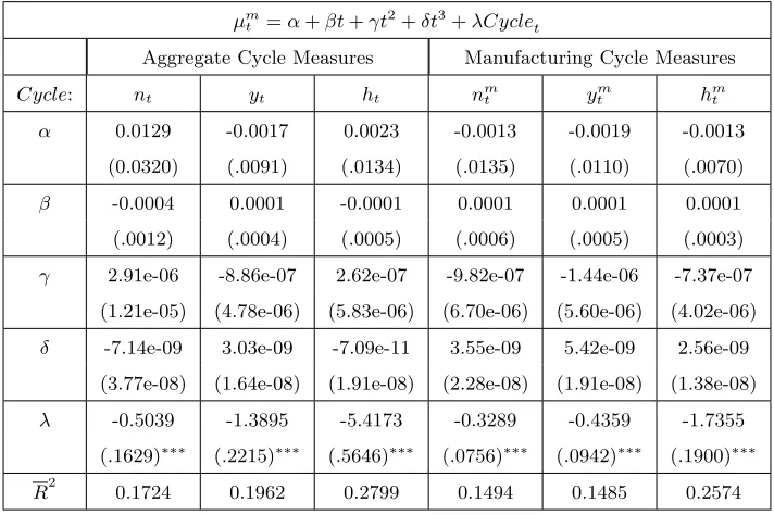
Using the same method as Bils (1987), we can provide a more rigorous examination of the cyclicality of the markup. This is done by regressing the HP detrended log markup index on a measure of the business cycle, time trends (𝑡, 𝑡2_{, and𝑡}3_{), and a constant. I also employ a}

Cochrane-Orcutt AR(1) correction in these regressions to adjust for serial correlation. For the business cycle measures, I use the output gap and hours ‘gap’,𝑦𝑡 and ℎ𝑡, as before. In

addi-tion, I also use an employment-based measure similar to what Bils uses, which is production-worker employment relative to the four surrounding years: 𝑛𝑡= ln(𝑁)−ln(𝑁−8𝑁−4𝑁+4𝑁+8).

These business cycle measures are estimated at the same level as the corresponding markup measure being tested. Namely, these levels are the manufacturing industry, the durables sector, and the nondurables sector, where these variables are denoted by superscripts of ‘𝑚’, ‘𝑑’, and ‘𝑛𝑑’ respectively. As a robustness check, aggregate business cycle measures are also tested6.

For the manufacturing markup, 𝜇𝑚_{, the results of tests of its cyclicality can be seen in}

Table 2. The most striking feature is that the coefficients on the business cycle measures–

whether aggregate or manufacturing–are highly negative and significant in every single case, providing strong evidence that the manufacturing markup is countercyclical. This gives more rigorous evidence of countercyclicality in addition to the visual observation of this fact. If we then consider the durables sector (Table 3), we find a contrasting result where all coefficients on the business cycle measures are statistically indistinguishable from zero, indicating that the durables markup is not countercyclical. On the other hand, the nondurables markup (Table 4) has highly negative and significant coefficients on all but one of the business cycle variables, indicating that the nondurables markup is in fact countercyclical. Therefore it seems that the observation that manufacturing’s markup is countercyclical is mainly being driven by the nondurables sector.

6

6

Determinants of the Manufacturing Markup

6.1 Model

Given that we have a new markup index for the manufacturing industry which is decreasing in trend from 1960:1 to 2007:3 and is also countercyclical, it is interesting to determine what is causing the markup to behave in this way. To answer this question, I modify the model proposed by Domowitz, Hubbard, and Petersen (1988), the main difference being that it is applied to time series data instead. Indeed, this paper is novel in that there seems to be a lack of work that has seriously examined the time series determinants of the markup.

Domowitz, Hubbard, and Petersen (1988) postulate that the markup will be dependent on a measure of market power since microeconomic theory suggests that firms with greater market power have more ability to set prices above marginal cost. Market power in turn will depend on both domestic and foreign competition. The former is often captured by concentration ratios, which is indicative of the degree of market power existing in an industry and therefore also affects what markups are charged. Yet foreign competition also affects the size of these markups, and there is a growing popular opinion that increased competition from overseas has reduced the market power of domestic markets, particularly in the manufacturing industry. This paper addresses this issue and attempts to quantify the role of both domestic and foreign competition on the behavior of the manufacturing markup over time. Specifically, the model I will implement is very similar to that employed by Marchetti (2002). This model states that the markup depends on a measure of the business cycle, domestic competition, foreign competition, and oil prices:

𝜇𝑚_𝑡 =𝜇𝑚+𝛽1𝑐𝑦𝑐𝑙𝑒𝑚𝑡 +𝛽2𝐶4𝑚𝑡 +𝛽3𝑖𝑚𝑝𝑚𝑡 +𝛽4𝑜𝑖𝑙𝑡+𝜀𝑚𝑡 (10)

where 𝑐𝑦𝑐𝑙𝑒𝑚

𝑡 is a measure of the business cycle or economic activity, 𝐶4𝑚𝑡 is a measure of

domestic competition (the concentration ratio for the 4 largest firms in the industry),𝑖𝑚𝑝𝑚 𝑡

is a measure of foreign competition (the share of goods produced in the industry that are imported), and 𝑜𝑖𝑙𝑡 is the oil price which is included to capture changes in non-labor costs.

main determinants of the manufacturing sector price-marginal cost markup. In addition to performing this multiple regression, I also examine how the model does when estimated with only one predictor at a time in order to get a better understanding of the contribution of each variable to the overall results.

6.2 Data

For the measure of the business cycle, 𝑛𝑚𝑡 , 𝑦𝑡𝑚, and ℎ𝑚𝑡 are used again, in the same way

as earlier defined. These business cycle variables can also be computed for the durables and nondurables sectors. For the measure of domestic competition, 𝐶4𝑚𝑡 , time series data

for concentration ratios is not readily available. The best available data on concentration ratios for the manufacturing sector is that recorded by the Census Bureau every 4 or 5 years, published at an annual frequency. The industrial organization literature bypasses the lack of time series data by focusing on cross-sectional analyzes or by implementing panel regressions with one or two years.

That being said, I proxy for𝐶4𝑚

𝑡 in two different ways. First, I take the Census Bureau

data for 13 surveys between 1954 and the present, and I then construct quarterly time se-ries. This is done by a simple linear interpolation7_{, assuming that the data points are for}

the first quarter of their respective years. Implementing this procedure results in the con-structed series𝐶4𝑙𝑖𝑛𝑚

𝑡 , which can be seen in Figure 7, where the dark points labeled in this

figure represent the actual data. The second proxy for domestic competition is profitability,

𝑝𝑟𝑜𝑓 𝑖𝑡𝑚

𝑡 , measured as the ratio of gross profits to total sales in the manufacturing industry

(BEA data). For instance, Sembenelli and Siotis (2003) also use profitability as a proxy for domestic competition, pointing out that the industrial organization literature has strong arguments as to why profitability can be used from a both a theoretical and empirical stand-point. Intuitively, higher profits are indicative of imperfect competition whereby a few firms in the industry are able to generate and sustain positive profits, which is invariably linked to higher markups. The series for𝑝𝑟𝑜𝑓 𝑖𝑡𝑚

𝑡 can be seen in Figure 8, and observation of this data

shows that profitability has been decreasing over time in a cyclical manner, particularly in the late 1990s and early 2000s where profitability fell sharply.

7

The share of imported manufactured goods,𝑖𝑚𝑝𝑚

𝑡 , is measured as the share of production

in manufacturing that is accounted for by imports (data from BEA), and this data can be seen in Figure 9. Although there have been a couple of small spurts of import share growth, overall this variable has steadily increased from a small share of roughly 5% of the industry in 1960 to a much larger share of 45% by 2005. This indicates how imports have become much more prevalent in the US manufacturing industry, and is a good candidate to explain how the markup has changed over time. Finally, data for 𝑜𝑖𝑙𝑡 is easily available8, and this

paper uses monthly data from the Federal Reserve of St. Louis which is then converted to quarterly data, plotted in Figure 10. From this figure we can see that oil prices were fairly stable until the early 1970s when they jumped up, and have continued to fluctuate up and down from the early 1980s onwards.

6.3 Estimation Methodology

The econometric issue with estimating (??) by OLS is the fact that these variables are inte-grated of different orders. When performing Dickey-Fuller and augmented Dickey-Fuller unit root tests, it turns out that𝑐𝑦𝑐𝑙𝑒𝑚

𝑡 is stationary, and that 𝜇𝑚𝑡 ,𝐶4𝑙𝑖𝑛𝑡𝑚,𝑝𝑟𝑜𝑓 𝑖𝑡𝑚𝑡 ,𝑖𝑚𝑝𝑚𝑡 , and

𝑜𝑖𝑙𝑡 are non-stationary9. In order to then estimate (??) given the issue of stationarity, I

im-plement the following two-stage procedure which is almost identical to Lettau and Ludvigson (2001), who use it to estimate the relationship between consumption and wealth.

In the first stage, we estimate a cointegrating regression with the non-stationary variables using dynamic OLS (DOLS) (see Stock and Watson (1993) for further details). Dynamic OLS involves estimating a standard OLS regression between the non-stationary variables, but then augmenting it with leads and lags of the first differences of the independent variables:

𝜇𝑚_𝑡 =𝛼+𝛽2𝐶4𝑚𝑡 +𝛽3𝑖𝑚𝑝𝑚𝑡 +𝛽4𝑜𝑖𝑙𝑡+ 𝑘

∑

𝑖=−𝑘

𝑏2Δ𝐶4𝑚𝑡−𝑖+ 𝑘

∑

𝑖=−𝑘

𝑏3Δ𝑖𝑚𝑝𝑚𝑡−𝑖+ 𝑘

∑

𝑖=−𝑘

𝑏4Δ𝑜𝑖𝑙𝑡−𝑖+𝜈𝑡𝑚

(11) In effect, the DOLS specification estimates the long run relationship between the I(1) vari-ables. It does this by adding an equal number of leads and lags10 of the first differenced

8

Note the absence of an ‘𝑚’ superscript on this variable, since this is the oil price that is faced by all firms. 9

Using a 5% level of significance. These variables are all𝐼(1). 10

variables to a standard OLS regression of the markup on domestic competition, the share of goods that are imported, and oil prices, to eliminate the effects of regressor endogeneity on the distribution of the least squares estimator. In other words, the two-stage DOLS tech-nique purges the error of endogenous components, ensuring that the remaining error term is orthogonal to the regressors. The coefficient estimates of the 𝛽s are now superconsistent as Stock (1987) argued. Therefore 𝛽2,𝛽3, and 𝛽4 from (??) are the same coefficients to be

estimated as in (??). In addition, we can also verify the existence of cointegration by checking that the residuals are stationary11_{. Following the cointegration regression we then move to}

the second stage, where we compute the cointegrating residuals,𝑟𝑡:

𝑟𝑡=𝜇𝑚𝑡 −𝛽2𝐶4𝑡𝑚−𝛽3𝑖𝑚𝑝𝑚𝑡 −𝛽4𝑜𝑖𝑙𝑡 (12)

which we can then regress on the stationary variables and a constant term to obtain the remaining coefficients:

𝑟𝑡=𝜇𝑚+𝛽1𝑐𝑦𝑐𝑙𝑒𝑚𝑡 +𝑢𝑡 (13)

where we have now estimated all of the coefficients from (??) accounting for the fact that the variables are integrated of different orders.

6.4 Results

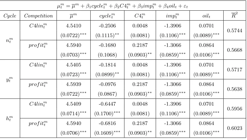
Undertaking this two-stage DOLS procedure then gives us the results presented in Table 5 for the manufacturing industry, where the model is estimated using multiple regressors. In addition, I also estimate the model separately with 𝐶4𝑚

𝑡 , 𝑝𝑟𝑜𝑓 𝑖𝑡𝑚𝑡 , 𝑖𝑚𝑝𝑚𝑡 , and 𝑜𝑖𝑙𝑡 as

individual regressors following the same estimation methodology as above, with the exception that the cointegrating regression is estimated with only one non-stationary variable at a time, including its respective leads and lags of first differences. These single predictor results can be seen in Table 6, which sheds light on how each variable contributes to the𝑅2 of the multiple regression model.

The most notable result in Table 5 is that the coefficient on 𝑖𝑚𝑝𝑚𝑡 is highly negative and

of𝑘= 8 is selected. 11

significant. In fact this variable achieves the highest𝑡-statistic out of all of the regressors with

𝑡=-15.21. This is true under every type of business cycle measure used, and is robust to the measure of domestic competition. Furthermore, Table 6 provides evidence that𝑖𝑚𝑝𝑚

𝑡 makes

the largest contribution to the behavior of the markup, since the𝑅2 ≈0.45 is the largest out of all of the single variable regressions. Oil prices make the next largest contribution to the

𝑅2, with the measures of domestic competition playing the least significant role. The fact that 𝑖𝑚𝑝𝑚𝑡 achieves the lowest 𝑝-value in both the single predictor and multiple regressions

as well as obtaining the highest 𝑅2, is of important economic significance. It tells us that foreign competition has been the main determinant behind the decline in the manufacturing markup from 1960:1 to 2007:3, out of all the variables considered in this paper. This is in keeping with what seems to be a popularly-held belief, that the increasing competitiveness of overseas manufacturers has had a large impact on US manufacturing. These findings confirm that foreign competition has in fact caused a decline in the degree of market power prevalent in domestic manufacturing, as indicated by the fall of the price-marginal cost markup.

The measure of domestic competition is statistically indistinguishable from zero with

𝐶4𝑙𝑖𝑛𝑚

𝑡 , but is positive and significant for𝑝𝑟𝑜𝑓 𝑖𝑡𝑚𝑡 , though not at the same level of significance

as𝑖𝑚𝑝𝑚𝑡 with𝑡=2.42. This confirms the idea that increasing market power in manufacturing

is associated with higher markups, and it appears that domestic competition has played some role in the behavior of the markup over the sample period. However it is interesting to note that the contribution (𝑅2 ≈0.39) of domestic competition to the movement of the markup is lower than with𝑖𝑚𝑝𝑚

𝑡 when single predictor regressions are considered.

When oil prices are tested individually in the model, we get negative and significant coefficients on𝑜𝑖𝑙𝑡 as Table 6 shows. Intuitively one would expect that higher oil prices lead

the business cycle variable is negative and significant in most cases–in both individual and multiple regressions–to varying levels of statistical significance. This reinforces the results of section 5, which suggest that the manufacturing markup moves in a countercyclical manner. One final aspect that is important to note is that the markup series in Figure 4 appears to have a ‘step’ in the series in the early 1980s. 𝐶4𝑙𝑖𝑛𝑚

𝑡 does not have a step12 (Figure 7),

and although𝑝𝑟𝑜𝑓 𝑖𝑡𝑚

𝑡 (Figure 8) is decreasing in a cyclical manner, there does not appear to

be any ‘jumps’ either, with the exception of one sharp fall in 2001-02. Hence these series do not seem to be driving the markup variable due to the reason of having a similar step in the early 1980s. Oil prices do jump upwards in the mid-to-late 1970s (Figure 10), but from the 1980s to the early 2000s have fluctuated around a roughly constant mean, and therefore also has a different trend from the markup. This may then lead one to conclude that 𝑖𝑚𝑝𝑚𝑡 is

the variable with the most impact on the markup if it has a similar step in the series around 1981. However, Figure 9 does not provide evidence of this: the share of imported goods in the manufacturing sector has steadily risen over the sample period, with the rate increasing faster mostly in the early 2000s. Certainly there is no step in the series in or around the early 1980s. Thus we can be satisfied that the import share is not the major determinant of the markup purely because it happens to match the step in the markup series. Indeed, we can be confident that the results obtained are reliable since the dynamic OLS equation in (??) takes care of trends in the data. This is true if we have non-stationary series (which are all 𝐼(1)) that are cointegrated, which is confirmed by the unit root tests performed at the outset of this exercise. Therefore we can be assured that DOLS takes care of the effects of any stochastic trends in the variables, and the results presented in Tables 5 and 6 can be safely interpreted.

In summary, it appears that increasing competition from overseas is the biggest determi-nant of the decline in the manufacturing industry’s markup from 1960 to 2007. Although domestic competition and oil prices have also played an important role, their impact is not as large as that achieved by the imported share of manufactured goods.

12

7

Determinants of the Durables, Nondurables Markups

7.1 Model

Given these manufacturing industry results, it is then of potential interest to examine these results at a slightly more disaggregated level to determine what sectors cause the markup to move in this way. I do this by re-estimating (??), but in a system of two equations for the durables and nondurables sectors:

𝜇𝑑_𝑡 =𝜇𝑑+𝛽𝑑,1𝑐𝑦𝑐𝑙𝑒𝑑𝑡+𝛽𝑑,2𝐶4𝑑𝑡 +𝛽𝑑,3𝑖𝑚𝑝𝑑𝑡 +𝛽𝑑,4𝑜𝑖𝑙𝑡+𝜀𝑑𝑡 (14)

𝜇𝑛𝑑𝑡 =𝜇𝑛𝑑+𝛽𝑛𝑑,1𝑐𝑦𝑐𝑙𝑒𝑛𝑑𝑡 +𝛽𝑛𝑑,2𝐶4𝑛𝑑𝑡 +𝛽𝑛𝑑,3𝑖𝑚𝑝𝑛𝑑𝑡 +𝛽𝑛𝑑,4𝑜𝑖𝑙𝑡+𝜀𝑛𝑑𝑡 (15)

where the same variables are stationary and non-stationary (which are𝐼(1)) as before. Data on𝑐𝑦𝑐𝑙𝑒𝑡and𝑖𝑚𝑝𝑡can be easily distinguished into durables and nondurables, whereas𝐶4𝑙𝑖𝑛𝑚𝑡

is only available for the manufacturing sector as a whole. Therefore I continue to use this variable measured at the manufacturing industry level in these disaggregated regressions, while𝑝𝑟𝑜𝑓 𝑖𝑡𝑡on the other hand can be measured at the durables and nondurables levels.

7.2 Estimation Methodology

The estimation technique for the disaggregated regressions is slightly different than for the single equation that I estimated for the entire manufacturing industry, since the goal is now to estimate (??) and (??) together. The reason for doing so, is that estimating (??) and (??) as a system allows for errors that may be correlated across equations, and also accounts for the fact that both equations share at least one independent variable. Thus I will estimate (??) and (??) using seemingly unrelated regressions (SUR) as an extension of the linear regression model.

estimates for 𝛽𝑖,2,𝛽𝑖,3, and𝛽𝑖,4 for 𝑖={𝑑, 𝑛𝑑}, which I can then compare using a standard

Wald test. Following this is the second stage where I compute the residuals𝑟𝑖,𝑡 similarly to

(??), which are also stationary according to unit root tests, providing evidence of cointegra-tion among the 𝐼(1) variables. Finally I regress these residuals on a constant and on the sector-specific business cycle variable, in a similar fashion to (??). This gives estimates of𝜇𝑖

and𝛽𝑖,1, which completes the set of parameters from (??) and (??) that we need to estimate.

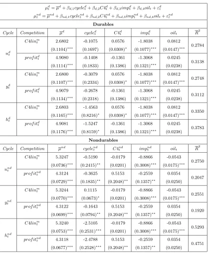
7.3 Results

The results of the SUR estimation for the durables and nondurables sectors can be seen in Table 7. Given our SUR setup we can also test the coefficients between the two sectors’ regressions. Specifically, I test𝐻0 :𝛽𝑑,𝑗 =𝛽𝑛𝑑,𝑗 for𝑗={2,3,4}under each proxy of domestic

competition using a simple Wald test, where the results can be seen in Table 8.

For the durables sector, the share of goods that are imported is highly negative and sig-nificant, and has the highest𝑡-statistic of𝑡=-16.74. Thus, the result that foreign competition is the major determinant of the markup holds especially true for the durables sector where competition from overseas has reduced the degree of market power existent in the domestic durables industry. For the proxies of domestic competition,𝐶4𝑙𝑖𝑛𝑚

𝑡 has had a small effect on

the markup, while profitability has had no impact. Thus domestic competition has not had as much impact on the behavior of the markup as foreign competition has. The final result of note from the durables sector is that the coefficient on 𝑐𝑦𝑐𝑙𝑒𝑑

𝑡 is only sometimes negative

and significant (and at the 10% level), indicating that the durables markup is at best only slightly countercyclical.

From the nondurables sector regressions, we see that𝑖𝑚𝑝𝑛𝑑

𝑡 is also negative and significant

in all cases, although the degree of significance varies between regressions. Out of the domestic competition measures, only𝑝𝑟𝑜𝑓 𝑖𝑡𝑛𝑑

𝑡 is ever positive and significant, but it appears to has as

much of an impact on the nondurables markup as foreign competition. While𝑖𝑚𝑝𝑛𝑑

𝑡 has had

and beverages. The Wald tests also show that the coefficients on domestic and foreign competition between the two sectors are not equal, indicating that the nature of competition differs between durables and nondurables. In particular, domestic competition seems to be slightly more important in nondurables than it is in the durables sector (highest𝑡-statistic for domestic competition in nondurables is𝑡=2.56 and in durables is 𝑡=1.87). Finally, it is interesting to observe that the coefficient on the business cycle indicates that the nondurables markup exhibits more evidence of countercyclicality than the durables markup, reinforcing earlier arguments in this paper.

8

Conclusion

The markup of price over marginal cost is an important concept in economics as a measure of the degree of market power that exists in an industry. Unfortunately, marginal cost is not directly observable from the data, so estimating the markup is not easy to do. Probably the most widely-used methodology of computing the markup is that based on Hall’s (1988) idea, whereby he manipulates the Solow Residual to be able to obtain an estimate of the markup. However this method has some limitations, which are ones that we have the ability to easily improve upon. Namely, the Hall framework implicitly assumes that labor can be freely adjusted at a fixed wage rate. Unfortunately this assumption is far from ideal, and as Mazumder (2009) argues, is an assumption that is easy to relax in a way that is a closer approximation to the real world. We then improve upon the measurement of marginal cost by implementing Bils (1987) idea of measuring marginal cost along any input, given firms optimally minimize costs. This new marginal cost measure is based on the variation of employees’ hours of work, and accounts for adjustment costs as well as the existence of overtime premia that is sometimes paid for an increase in hours worked. One of the advantages of obtaining this new marginal cost variable, is that it allows us to then derive a markup index in a straightforward way.

why the markup has decreased in trend from the 1960s to present, this paper then examines potential determinants of the price-marginal cost markup. And the conclusion is clear that the markup for US manufacturing is primarily driven by foreign competition, and while do-mestic competition is also important, it has played much less of a role. In particular, the effect of foreign competition can be observed mostly in the durables sector. This is in keeping with the popular belief that competition from overseas has had a large impact on US manu-facturing, and this paper provides evidence that the degree of market power has been reduced in this industry by the rising share of imported goods. Future research is needed to extend upon this result by also examining the relationship between oil prices and marginal cost at greater detail, and by exploring the different nature of competition that exists between the durables and nondurables sectors.

References

[1] Bils, M., 1987. “The cyclical behavior of marginal cost and price.”American Economic Review 77, 838-855.

[2] Bresnahan, T.F., 1989. “Empirical studies of industries with market power.” in Schmalensee, R., Willing, R. (Ed.), Handbook of Industrial Organization, 1011-1057. Elsevier.

[3] Caballero, R.J., Lyons, R.K., 1992. “External effects in U.S. procyclical productivity.”

Journal of Monetary Economics 29, 209-225.

[4] Domowitz, I., Hubbard, R.G., Petersen, B.C., 1988. “Market structure and cyclical fluctuations in U.S. manufacturing.”Review of Economics and Statistics 70, 55-66.

[5] Eden, B., Griliches, Z., 1993. “Productivity, market power, and capacity utilization when spot markets are complete.”American Economic Review 83, 219-223.

[7] Hall, R.E., 1986. “Market structure and macro fluctuations.”Brookings Papers on Eco-nomic Activity 2, 285-322.

[8] Hall, R.E., 1988. “The relation between price and marginal cost in U.S. industry.” Jour-nal of Political Economy 96, 921-947.

[9] Hylleberg, S., Joergensen, R.W. 1998. “A note on the estimation of markup pricing in manufacturing.” University of Aarhus, School of Economics and Management, Eco-nomics Working Paper 6.

[10] Lettau, M., Ludvigson, S., 2001. “Consumption, aggregate wealth, and expected stock returns.” Journal of Finance 56, 815-849.

[11] Lewis, H.G., 1969. “Employer interests in employee hours of worked.” Cuadernos de Economia 18, 38-54.

[12] Marchetti, D.J., 2002. “Markup and the business Cycle: evidence from Italian manufac-turing branches.” Open Economies Review 13, 87-103.

[13] Mazumder, S., 2009. “The New Keynesian Phillips Curve and the Cyclicality of Marginal Cost.”Forthcoming.

[14] Oi, W., 1962., “Labor as a quasi-fixed factor.”Journal of Political Economy 70, 538-555.

[15] Roeger, W., 1995. “Can imperfect competition explain the difference between primal and dual productivity measures? Estimates for U.S. manufacturing.” Journal of Political Economy 103, 316-330.

[16] Rotemberg, J.,J., Woodford, M., 1990. “Cyclical markups: theories and evidence.”

NBER Working Paper 3534.

[17] Rotemberg, J.J., Woodford, M., 1999. “The cyclical behavior of prices and costs.” in Taylor, J.B., Woodford, M. (Ed.), The Handbook of Macroeconomics, edition 1, volume 1, pp. 1051-1135. Amsterdam: North-Holland.

[18] Sembenelli, A., Siotis, G., 2005. “Foreign direct investment, competitive pressure and spillovers. An empirical analysis of Spanish firm level data.” CEPR Discussion Papers

[19] Shapiro, M.D., 1987. “Measuring market power in U.S. industry.” Cowles Foundation Discussion Paper 828.

[20] Stock, J.H., 1987. “Asymptotic properties of least squares estimators of cointegrating vectors.” Econometrica 55, 1035-1056.

[21] Stock, J.H., Watson, M.W., 1993. “A simple estimator of cointegrating vectors in higher order integrated systems.”Econometrica 61, 783-820.

Table 1: 𝜈(𝐻) Regressions

𝜈(𝐻) =𝑎+𝑏𝐻 𝜈(𝐻) =𝑎+𝑏𝐻+𝑐𝐻2

a b a b c

Coefficient -.9760154 .0264254 8.396427 -.4361621 .0057049 Standard Error (.0264964)∗∗∗ _(.0006491)∗∗∗ _(.949713)∗∗∗ _(.0469388)∗∗∗ _(.0005796)∗∗∗

𝑅2 0.8917 0.9228

Table 2: Cyclicality of Manufacturing Markup

𝜇𝑚

𝑡 =𝛼+𝛽𝑡+𝛾𝑡

2 +𝛿𝑡3

+𝜆𝐶𝑦𝑐𝑙𝑒_𝑡

Aggregate Cycle Measures Manufacturing Cycle Measures

𝐶𝑦𝑐𝑙𝑒: 𝑛𝑡 𝑦𝑡 ℎ𝑡 𝑛𝑚𝑡 𝑦𝑚𝑡 ℎ𝑚𝑡

𝛼 0.0129 -0.0017 0.0023 -0.0013 -0.0019 -0.0013

(0.0320) (.0091) (.0134) (.0135) (.0110) (.0070)

𝛽 -0.0004 0.0001 -0.0001 0.0001 0.0001 0.0001

(.0012) (.0004) (.0005) (.0006) (.0005) (.0003)

𝛾 2.91e-06 -8.86e-07 2.62e-07 -9.82e-07 -1.44e-06 -7.37e-07 (1.21e-05) (4.78e-06) (5.83e-06) (6.70e-06) (5.60e-06) (4.02e-06)

𝛿 -7.14e-09 3.03e-09 -7.09e-11 3.55e-09 5.42e-09 2.56e-09 (3.77e-08) (1.64e-08) (1.91e-08) (2.28e-08) (1.91e-08) (1.38e-08)

𝜆 -0.5039 -1.3895 -5.4173 -0.3289 -0.4359 -1.7355

(.1629)∗∗∗ (.2215)∗∗∗ (.5646)∗∗∗ (.0756)∗∗∗ (.0942)∗∗∗ (.1900)∗∗∗

𝑅2 0.1724 0.1962 0.2799 0.1494 0.1485 0.2574

∗_,∗∗_{, and}∗∗∗ _{denote 10, 5, and 1% levels of significance respectively. Also, the (log) markup variable is HP}

Table 3: Cyclicality of Durables Markup

𝜇𝑑

𝑡 =𝛼+𝛽𝑡+𝛾𝑡

2 +𝛿𝑡3

+𝜆𝐶𝑦𝑐𝑙𝑒_𝑡

Aggregate Cycle Measures Durables Cycle Measures

𝐶𝑦𝑐𝑙𝑒: 𝑛𝑡 𝑦𝑡 ℎ𝑡 𝑛𝑑𝑡 𝑦𝑡𝑑 ℎ𝑑𝑡

𝛼 -0.0246 0.0026 0.0077 0.0027 0.0040 0.0027

(.0953) (.0276) (.0646) (.0291) (.0283) (.0291)

𝛽 0.0008 -0.0001 -0.0002 -0.0001 -0.0001 -0.0001

(.0033) (.0013) (.0024) (.0014) (.0014) (.0014)

𝛾 -8.41e-06 6.80e-07 1.90e-06 1.16e-06 1.32e-06 1.16e-06 (3.30e-05) (1.64e-05) (2.56e-05) (1.76e-05) (1.67e-05) (1.76e-05)

𝛿 2.59e-08 -1.50e-09 -4.74e-09 -3.85e-09 -3.55e-09 -3.85e-09 (1.01e-07) (5.56e-08) (8.01e-08) (6.01e-08) (5.63e-08) (6.01e-08)

𝜆 -0.4985 -0.9189 -0.9513 -0.2221 -0.1296 -0.2221

(.4949) (.8894) (2.9008) (.1904) (.2615) (.1904)

𝑅2 0.0700 0.0689 0.0612 0.0713 0.0624 0.0613

Table 4: Cyclicality of Nondurables Markup

𝜇𝑛𝑑𝑡 =𝛼+𝛽𝑡+𝛾𝑡

2

+𝛿𝑡3+𝜆𝐶𝑦𝑐𝑙𝑒𝑡

Aggregate Cycle Measures Nondurables Cycle Measures

𝐶𝑦𝑐𝑙𝑒: 𝑛𝑡 𝑦𝑡 ℎ𝑡 𝑛𝑛𝑑𝑡 𝑦𝑡𝑛𝑑 ℎ𝑛𝑑𝑡

𝛼 0.0369 -0.0035 -0.0021 0.0004 0.0016 -0.0062

(.0589) (.0190) (.0366) (.0206) (.0221) (.0113)

𝛽 -0.0011 0.0001 0.0001 -0.0001 -0.0001 0.0003

(.0021) (.0009) (.0013) (.0010) (.0011) (.0006)

𝛾 0.0000 -1.48e-06 -1.04e-06 2.03e-06 9.42e-07 -3.38e-06 (.0000) (1.15e-05) (1.42e-05) (1.21e-05) (1.26e-05) (7.62e-06)

𝛿 -2.93e-08 4.67e-09 3.61e-09 -8.97e-09 -3.31e-09 1.16e-08 (6.66e-08) (3.81e-08) (4.43e-08) (4.09e-08) (4.16e-08) (2.65e-08)

𝜆 -0.3370 -1.5507 -7.7204 -0.7271 -0.4655 -5.0121

(.3623) (.6604)∗∗ _(1.7676)∗∗∗ _(.3685)∗∗ _(.2760)∗ _(.2542)∗∗∗

Table 5: Determinants of Manufacturing Markup-2 stage DOLS, Multiple

Regressions

𝜇𝑚

𝑡 =𝜇𝑚+𝛽1𝑐𝑦𝑐𝑙𝑒𝑚_𝑡 +𝛽2𝐶4𝑚_𝑡 +𝛽3𝑖𝑚𝑝𝑚_𝑡 +𝛽4𝑜𝑖𝑙𝑡+𝜀𝑡

Cycle Competition 𝜇𝑚 𝑐𝑦𝑐𝑙𝑒𝑚𝑡 𝐶4𝑚𝑡 𝑖𝑚𝑝𝑚𝑡 𝑜𝑖𝑙𝑡 𝑅

2

𝑛𝑚 𝑡

𝐶4𝑙𝑖𝑛𝑚

𝑡 4.5410 -0.2506 0.0048 -1.3906 0.0701

0.5744 (0.0722)∗∗∗ _(0.1115)∗∗ _{(0.0081) (0.1106)}∗∗∗ _(0.0089)∗∗∗

𝑝𝑟𝑜𝑓 𝑖𝑡𝑚

𝑡 4.5940 -0.1680 0.2187 -1.3066 0.0864

0.5668 (0.0703)∗∗∗ _{(0.1068) (0.0903)}∗∗ _(0.0859)∗∗∗ _(0.0106)∗∗∗

𝑦𝑚 𝑡

𝐶4𝑙𝑖𝑛𝑚

𝑡 4.5405 -0.1814 0.0048 -1.3906 0.0701

0.5717 (0.0723)∗∗∗ _(0.0899)∗∗ _{(0.0081) (0.1106)}∗∗∗ _(0.0089)∗∗∗

𝑝𝑟𝑜𝑓 𝑖𝑡𝑚

𝑡 4.5939 -0.0976 0.2187 -1.3066 0.0864

0.5638 (0.0722)∗∗∗ (0.0867) (0.0903)∗∗ (0.0859)∗∗∗ (0.0106)∗∗∗

ℎ𝑚 𝑡

𝐶4𝑙𝑖𝑛𝑚

𝑡 4.5409 -0.6447 0.0048 -1.3906 0.0701

0.5956 (0.0714)∗∗∗ (0.1700)∗∗∗ (0.0081) (0.1106)∗∗∗ (0.0089)∗∗∗

𝑝𝑟𝑜𝑓 𝑖𝑡𝑚𝑡 4.5940 -0.6816 0.2187 -1.3066 0.0864

Table 6: Determinants of Manufacturing Markup-2 stage DOLS, Single

Variable Regressions

(a)𝜇𝑚

𝑡 =𝜇𝑚+𝛽𝑐𝑦𝑐𝑙𝑒𝑚𝑡 +𝛾𝐶4𝑚𝑡 +𝜀𝑡

Cycle 𝜇𝑚 𝑐𝑦𝑐𝑙𝑒𝑚𝑡 𝐶4𝑚𝑡 𝑅

2

𝑛𝑚 𝑡

4.2617 -0.6496 -0.0682

0.3758 (0.3113)∗∗∗ _(0.1516)∗∗∗ _(0.0105)∗∗∗

𝑦𝑚 𝑡

4.2605 -0.4383 -0.0682

0.3736 (0.3191)∗∗∗ _(0.1083)∗∗∗ _(0.0105)∗∗∗

ℎ𝑚 𝑡

4.2609 -1.0547 -0.0682

0.3810 (0.3280)∗∗∗ _(0.1987)∗∗∗ _(0.0105)∗∗∗

(b)𝜇𝑚𝑡 =𝜇𝑚+𝛽𝑐𝑦𝑐𝑙𝑒𝑚𝑡 +𝛾𝑝𝑟𝑜𝑓 𝑖𝑡𝑚𝑡 +𝜀𝑡

Cycle 𝜇𝑚 _{𝑐𝑦𝑐𝑙𝑒}𝑚

𝑡 𝑝𝑟𝑜𝑓 𝑖𝑡𝑚𝑡 𝑅

2

𝑛𝑚𝑡

4.4635 -0.3652 0.4520

0.3933 (0.3582)∗∗∗ _(0.1389)∗∗∗ _(0.0706)∗∗∗

𝑦𝑚𝑡

4.4629 -0.1675 0.4520

0.3907 (0.3639)∗∗∗ _{(0.1023) (0.0706)}∗∗∗

ℎ𝑚 𝑡

4.4620 -0.9146 0.4520

0.4032 (0.3813) (0.1821)∗∗∗ _(0.0706)∗∗∗

(c)𝜇𝑚

𝑡 =𝜇𝑚+𝛽𝑐𝑦𝑐𝑙𝑒𝑚𝑡 +𝛾𝑖𝑚𝑝𝑚𝑡 +𝜀𝑡

Cycle 𝜇𝑚 _{𝑐𝑦𝑐𝑙𝑒}𝑚

𝑡 𝑖𝑚𝑝𝑚𝑡 𝑅

2

𝑛𝑚 𝑡

4.7956 -0.5210 -0.7011

0.4531 (0.2342)∗∗∗ (0.1253)∗∗∗ (0.0602)∗∗∗

𝑦𝑚𝑡

4.7948 -0.2666 -0.7011

0.4450 (0.2393)∗∗∗ (0.0917)∗∗∗ (0.0602)∗∗∗

ℎ𝑚𝑡

4.7953 -0.7938 -0.7011

0.4562 (0.2457)∗∗∗ (0.1673)∗∗∗ (0.0602)∗∗∗

(d)𝜇𝑚

𝑡 =𝜇𝑚+𝛽𝑐𝑦𝑐𝑙𝑒𝑚𝑡 +𝛾𝑜𝑖𝑙𝑡+𝜀𝑡

Cycle 𝜇𝑚 𝑐𝑦𝑐𝑙𝑒𝑚𝑡 𝑜𝑖𝑙𝑡 𝑅

2

𝑛𝑚 𝑡

4.7716 -0.6366 -0.0586

0.4183 (0.2799)∗∗∗ _(0.1572)∗∗∗ _(0.0066)∗∗∗

𝑦𝑚 𝑡

4.7709 -0.3930 -0.0586

0.4032 (0.2804)∗∗∗ _(0.1170)∗∗∗ _(0.0066)∗∗∗

ℎ𝑚 𝑡

4.7707 -1.0415 -0.0586

Table 7: Determinants of Durables, Nondurables Markup-SUR

𝜇𝑑

𝑡 =𝜇𝑑+𝛽𝑑,1𝑐𝑦𝑐𝑙𝑒𝑑_𝑡 +𝛽𝑑,2𝐶4_𝑡𝑑+𝛽𝑑,3𝑖𝑚𝑝𝑑_𝑡 +𝛽𝑑,4𝑜𝑖𝑙𝑡+𝜀𝑑𝑡

𝜇𝑛𝑑𝑡 =𝜇𝑛𝑑+𝛽𝑛𝑑,1𝑐𝑦𝑐𝑙𝑒𝑛𝑑𝑡 +𝛽𝑛𝑑,2𝐶4𝑛𝑑𝑡 +𝛽𝑛𝑑,3𝑖𝑚𝑝𝑛𝑑𝑡 +𝛽𝑛𝑑,4𝑜𝑖𝑙𝑡+𝜀𝑛𝑑𝑡

Durables

Cycle Competition 𝜇𝑑 _{𝑐𝑦𝑐𝑙𝑒}𝑑

𝑡 𝐶4𝑑𝑡 𝑖𝑚𝑝𝑑𝑡 𝑜𝑖𝑙𝑡 𝑅

2

𝑛𝑑 𝑡

𝐶4𝑙𝑖𝑛𝑚

𝑡 2.6802 -0.1075 0.0576 -1.8038 0.0812

0.2784 (0.1104)∗∗∗ _{(0.1697) (0.0308)}∗ _(0.1077)∗∗∗ _(0.0147)∗∗∗

𝑝𝑟𝑜𝑓 𝑖𝑡𝑑𝑡 4.9080 -0.1408 -0.1361 -1.3068 0.0245

0.3138 (0.1114)∗∗∗ (0.1833) (0.1386) (0.1321)∗∗∗ (0.0238)

𝑦𝑑𝑡

𝐶4𝑙𝑖𝑛𝑚𝑡 2.6800 -0.3079 0.0576 -1.8038 0.0812

0.2748 (0.1107)∗∗∗ (0.2334) (0.0308)∗ (0.1077)∗∗∗ (0.0147)∗∗∗

𝑝𝑟𝑜𝑓 𝑖𝑡𝑑

𝑡 4.9079 -0.2678 -0.1361 -1.3068 0.0245

0.3112 (0.1134)∗∗∗ _{(0.2318) (0.1386) (0.1321)}∗∗∗ _(0.0238)

ℎ𝑑𝑡

𝐶4𝑙𝑖𝑛𝑚𝑡 2.6803 -1.4563 0.0576 -1.8038 0.0812

0.3350 (0.1165)∗∗∗ _(0.8216)∗ _(0.0308)∗ _(0.1077)∗∗∗ _(0.0147)∗∗∗

𝑝𝑟𝑜𝑓 𝑖𝑡𝑑

𝑡 4.9081 -1.5247 -0.1361 -1.3068 0.0245

0.3783 (0.1176)∗∗∗ _(0.8159)∗ _{(0.1386) (0.1321)}∗∗∗ _(0.0238)

Nondurables

Cycle Competition 𝜇𝑛𝑑 _{𝑐𝑦𝑐𝑙𝑒}𝑛𝑑

𝑡 𝐶4𝑛𝑑𝑡 𝑖𝑚𝑝𝑛𝑑𝑡 𝑜𝑖𝑙𝑡 𝑅

2

𝑛𝑛𝑑𝑡

𝐶4𝑙𝑖𝑛𝑚𝑡 5.3247 -0.5190 -0.0179 -0.8866 -0.0543

0.2750 (0.0736)∗∗∗ (0.2415)∗∗ (0.0201) (0.3008)∗∗∗ (0.0175)∗∗∗

𝑝𝑟𝑜𝑓 𝑖𝑡𝑛𝑑𝑡 4.3124 -0.3625 0.5153 -0.2559 0.0354

0.2047 (0.0729)∗∗∗ _(0.1835)∗∗ _(0.2048)∗∗ _(0.1357)∗∗ _(0.0250)

𝑦𝑡𝑛𝑑

𝐶4𝑙𝑖𝑛𝑚𝑡 5.3244 0.1115 -0.0179 -0.8866 -0.0543

0.2551 (0.0770)∗∗∗ _(0.0673)∗ _{(0.0201) (0.3008)}∗∗∗ _(0.0175)∗∗∗

𝑝𝑟𝑜𝑓 𝑖𝑡𝑛𝑑

𝑡 4.3122 -0.1643 0.5153 -0.2559 0.0354

0.1920 (0.0699)∗∗∗ _(0.0794)∗∗ _(0.2048)∗∗ _(0.1357)∗∗ _(0.0250)

ℎ𝑛𝑑 𝑡

𝐶4𝑙𝑖𝑛𝑚

𝑡 5.3240 -2.5105 -0.0179 -0.8866 -0.0543

0.5293 (0.0753)∗∗∗ _(0.2531)∗∗∗ _{(0.0201) (0.3008)}∗∗∗ _(0.0175)∗∗∗

𝑝𝑟𝑜𝑓 𝑖𝑡𝑛𝑑

𝑡 4.3118 -2.4788 0.5153 -0.2559 0.0354

Table 8: Wald Test on Coefficients between Durables & Nondurables

Cointegrating Regressions

𝜇𝑑

𝑡 =𝛼𝑑+𝛽𝑑,2𝐶4𝑑𝑡 +𝛽𝑑,3𝑖𝑚𝑝𝑑𝑡+𝛽𝑑,4𝑜𝑖𝑙𝑡+𝐿𝑒𝑎𝑑𝑠, 𝐿𝑎𝑔𝑠

𝜇𝑛𝑑

𝑡 =𝛼𝑛𝑑+𝛽𝑛𝑑,2𝐶4𝑛𝑑_𝑡 +𝛽𝑛𝑑,3𝑖𝑚𝑝𝑛𝑑_𝑡 +𝛽𝑛𝑑,4𝑜𝑖𝑙𝑡+𝐿𝑒𝑎𝑑𝑠, 𝐿𝑎𝑔𝑠

Measure of𝐶4𝑚 𝑡

𝐻0 𝐶4𝑙𝑖𝑛𝑚𝑡 𝑝𝑟𝑜𝑓 𝑖𝑡{ 𝑑,𝑛𝑑}

𝑡

𝛽𝑑,2=𝛽𝑛𝑑,2 0.0403∗∗ 0.0014∗∗∗

𝛽𝑑,3=𝛽𝑛𝑑,3 0.0013∗∗∗ 0.0146∗∗

𝛽𝑑,4=𝛽𝑛𝑑,4 0.0000∗∗∗ 0.7987

31 

32 

33 

34 

35