Munich Personal RePEc Archive
Looking behind Granger causality
Chen, Pu and Hsiao, Chih-Ying
Melbourne University, University of Technology Sydney
September 2010
Online at
https://mpra.ub.uni-muenchen.de/24859/
Looking Behind Granger Causality
Pu Chen
∗and Chih-Ying Hsiao
†September 8, 2010
Abstract
Granger causality as a popular concept in time series analysis is widely ap-plied in empirical research. The interpretation of Granger causality tests in a cause-effect context is, however, often unclear or even controversial, so that the causality label has faded away. Textbooks carefully warn that Granger causal-ity does not imply true causalcausal-ity and preferably refer the Granger causalcausal-ity test to a forecasting technique. Applying theory of inferred causation, we develop in this paper a method to uncover causal structures behind Granger causality. In this way we re-substantialize the causal attribution in Granger causality through providing an causal explanation to the conditional depen-dence manifested in Granger causality.
KEYWORDS: Granger Causality, Time Series Causal Model, Graphical Model
JEL CLASSIFICATION SYSTEM FOR JOURNAL ARTICLES: C1, E3
∗Corresponding author, Melbourne University, E-Mail: [email protected]. This research
was supported by the Faculty Research Grant of Faculty of Economics and Business of Melbourne University.
Contents
1 Introduction 3
2 Time Series Causal Models 4
3 Granger Causality in TSCMs 7
3.1 Granger causality . . . 7
3.2 Conditional Dependance and Conditional Independence in DAG . . . 8
3.3 Granger Casuality in TSCM . . . 8
3.4 From Partial DAGs to Directed Graphs for Granger Causality . . . . 9
4 Some Examples 11
5 Looking Behind Granger Causality between Wages and Prices 19
1
Introduction
Since the publication of the influential seminar paper of TESTING FOR
CAUSAL-ITY: A Personal Viewpoint by C. W. J. Granger in 19801, Granger causality is
widely applied in empirical research on economic time series. Technically, the
Granger causality test is a method for determining whether one time series is useful in forecasting another. Since predictability is a central feature of causal attribution, Granger causality is interpreted often also in cause-effect context. In analyzing eco-nomic time series, many researchers are keen to find a story that one time series Granger causes the other but not the other way around. In practice, however, it happens often that either two economic time series are Granger cause to each other or they are non-Granger cause to each other. This phenomenon greatly weakens the power of Granger causality in investigating cause-effect relations. Therefore, text books usually state carefully that Granger causality does not imply true causality. Nevertheless, Granger causality does imply conditional dependence. Regarding to
dependence and causality, Reichenbach’s principle2 states that every dependence
requires a causal explanation. We ask a question: what is the causal explanation behind Granger causality?
The objective of this paper is to provide an answer to the question: what is the causal mechanism that generates Granger causality. According to Reichenbach’s principle, we assume that for a given Granger causality test result between some time series, there exists a causal structure among the time series variables, which leads the Granger causality relation between the time series. Applying the method
of inferred causation3, we can infer the causal structure from the time series data.
Based on the inferred causal structure among the time series, the Granger causality relation between the time series can be derived. We take the causal structure as the mechanism that generates the Granger causality relation. In this way we provide a causal explanation to the conditional dependence revealed by the Granger causality test result.
The paper is organized as follows.
In Section 2, we present a graphical causal model for time series called time series causal model (TSCM), which builds a basis for analyzing causal structures among time series. We discuss shortly how the method of inferred causation can be used to uncover the causal structures implied in time series data. In Section 3 we discuss Granger causality in TSCMs and derive graphical rules to transform the causal graph of a TSCM to the graphs presenting the bivariate Granger causality relation as well as the multivariate Granger causality relation. In Section 4 we demonstrate through examples how to derive Granger causality relations in TSCMs and show how the derived Granger causality relations matche the corresponding Granger causality test results. Section 5 contains an empirical application, where we show how our method can be applied to analyze the mutual Granger causality relation between wage inflation and price inflation. The last section concludes.
1
See Granger (1980) for more details.
2
See Reichenbach (1956) and for more details.
3
2
Time Series Causal Models
The basic idea of Granger causality is quite simple. Suppose that we have three
sets of time series Wt, Yt, and Zt, and that we have a prediction of Yt+1 based on
lagged values of Yt and Zt. Then we want to improve the prediction by including
the lagged values ofWt. If the second prediction is better, then the lagged values of
Wt contain information for forecastingYt+1 that is not in the past of Yt and Zt. In
this case we sayWt Granger causesYt. IfZt includes already a large set of carefully
chosen explanatory variables, Wt seems to contain certain unique information for
predictingYt+1. This justifies why we say Wt Granger causes Yt. If Zt is empty, we
refer it to bivariate Granger causality, otherwise to multivariate Granger causality4.
Suppose that two time series, say Wt and Yt, are mutually Granger causal to
each other. We want to give a causal explanation that leads to the dependence implied by the Granger causality test. The mutual Granger causality relation may be an effect that these two time series are indeed causal to each other. It may also be that the two time series are driven by one or more common cause processes, say
Zt, at different lags. Therefore to give a causal explanation to the Granger causality
relation we need to take all these potentially relevant time series into account.
Let the number of all relevant variables including Wt, Yt and Zt be N. We
collect these N time series together and denote them by Xt. We view the N time
series with T observations as realizations of a set of N T random variables. We
want to uncover the causal relations among theseN T variables in order to give the
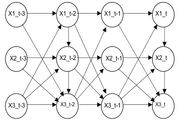
”Granger causality” a causal explanation. According to theory of inferred causation, any causal structure can be represented by a directed acyclic graph (DAG) in which arrows indicate the causal orders (See Hoover (2010) for more details). A causal
model for N T variables is a DAG with N T nodes (See Fig. 1 for an example with
N = 3 and T = 4.). To find out the causal structure among these N T variables
is to infer the arrows in the causal graph from data. If the joint distribution of the variables is normal, the DAG model can be equivalently presented as a system of linear recursive structural equations as follows (See Pearl (2000) p. 27 for more details.).
X1_t-1
X2_t-1
X3_t-1
X1_t
X2_t
X3_t
X1_t-3
X2_t-3
X3_t-3
X1_t-2
X2_t-2
[image:5.612.209.388.477.600.2]X3_t-2
Figure 1: TSCM with N = 3 andT = 4
AX =ǫ, (2.1)
whereA is an N T ×N T lower triangular matrix,X is a random vector containing
all the N T random variables in their causal order, ǫ∼ N(0, D) is an N T vector of
4
independent residuals,D is a diagonal matrix, implying thatǫi,t andǫj,t−τ are
inde-pendent. Although equation (2.1) is called a system of equations representing the
causal relations amongX, it is not yet specified at all. It is the order of the elements
inX and the restrictions on the corresponding parameter matrixA that specify the
causal relations among variables in X. From observations of X to infer the causal
order in the elements of X and to infer the restrictions on the corresponding A is
the task of causal analysis using theory of inferred causation. The theory of inferred causation is a graph-theoretic and statistical approach to causation. Pearl (2000) gives a systematic and general account of the theory of inferred causation. Spirtes, Glymour, and Scheines (2000) provide detailed techniques of the theory of inferred causation. Since the theory of inferred causation is a statistical approach and we
have only one observation for each random element Xit, many restrictions have to
be imposed on the recursive model (2.1) to make it statistically assessable.
Temporal information provides a nature causal order. Therefore, the recursive structural model must follow the temporal order. Consequently, we can write the recursive system as follows:
A11 0 . . . 0
A21 A22 0
..
. . .. ...
AT1 AT2 . . . AT T
X1 X2 .. . XT = ǫ1 ǫ2 .. . ǫT , (2.2)
whereXt= (X1t, X2t, ..., XN t)′ fort= 1,2, ...T is the random vector at timet.5 The
system in (2.2) contains still too many parameters to be analyzed statistically. We need to impose further constraints on the parameters. One reasonable constraining assumption is that the causal structure is time invariant: the causal relations
be-tween variables at time points t and s is the same as the causal relations between
variables at time pointst+τ ands+τ. We call it the time invariant causal structure
constraint. Another reasonable constraining assumption is the time-finite causal
in-fluence constraint that Xt may have a causal influence on Xt+τ only when τ ≤ p,
wherep <∞ is a given positive integer6.
Under the assumptions of the temporal causal constraint, the time-invariant causal structure constraint and the time-finite causal influence constraint, the linear
recursive system (2.2) with p= 2 can be written as follows
A0 0 . . . 0
A1 A0 0 . . . 0
A2 A1 A0 0 . . . 0
0 . .. ... ... ... ...
..
. 0 A2 A1 A0 0
0 . . . 0 A2 A1 A0
X1 X2 ... XT−1
XT = ǫ1 ǫ2 ... ǫT−1
ǫT . (2.3)
The parameter matricesA1, A2, ...Ap att-th row in equation (2.3) present the causal
influence of Xt−1, ...Xt−p on Xt and A0 is the contemporaneous causal influence
among the elements of Xt. The time-finite constraint implies that in each row all
5
In the model above we have assumed that the random process started at t = 1.
6
the parameter sub-matrices left to Ap are zero. We call the causal model in (2.3) a
time series causal model (TSCM).
Since the coefficient matrix in (2.3) is a lower triangular matrix, A0 must be a
lower triangular matrix too. Equation (2.3) can be reformulated as follows7
A0Xt+A1Xt−1 +...ApXt−p =ǫt, for t=p+ 1, p+ 2, ..., T. (2.4)
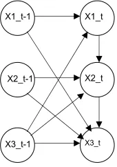
Corresponding to the TSCM in (2.4) we can represent the DAG for a TSCM through
a partial DAG, namely only through the nodes for (Xt, Xt−1, ..., Xt−p) and arrows
heading at the nodes representing Xt (See Fig. 2 for a TSCM with N = 3 and
p= 1.). This implies that instead of a DAG with T N nodes we need now only to
consider a partial DAG with (p+ 1)N nodes.
X1_t-1
X2_t-1
X3_t-1
X1_t
X2_t
[image:7.612.256.341.217.338.2]X3_t
Figure 2: A Partial DAG of a TSCM with N = 3 and p= 1
The parameter matrices (A0, A1, ..., Ap) correspond to the arrows in the partial
DAG. Ak(i, j)6= 0 corresponds to the arrow from the node Xj,t−k to the node Xit.
Ak(i, j) = 0 means there is no arrow from the node Xj,t−k to the node Xit. The
nonzero elements in the parameter matrices determine the topology of the partial causal graph. From sample information to infer the topology of the underlying DAG is the main research issue in the theory of inferred causation. Spirtes et al. (2000) provides a systematic discussion of the techniques and algorithms used to infer DAGs from sample information. A fundamental technique is the establishment of an isomorphism between DAGs and the conditional independence relationships encoded in joint probability distribution of the variables, such that the sample information can be used to recover the DAGs. Given a set of data generated from a DAG model, a statistical procedure can principally identify all the conditional independencies. However, the statistical procedure cannot tell whether this kind of independencies are due to the absence of some arrows in the DAG of the causal model or due to some particularly chosen parameter values in the DAG model such that the corresponding arrows in this case imply the conditional independencies. To rule out this ambiguity, Pearl (2000) assumes that all the identified conditional independencies are due to
absence of arrows in the DAG of the causal model. This assumption is calledstability
condition in Pearl (2000). In Spirtes et al. (2000) it is calledf aithf ulnesscondition.
This assumption is therefore important for interpreting the conditional dependence and independence as causal relations.
7
In our paper we assume generally that TSCMs as a special class of DAG models
satisfy the f aithf ulness condition. Spirtes et al. (2000)8 present several consistent
learning algorithms to uncover DAGs from independent data. Chen (2010) present a procedure to uncover partial DAGs for TSCMs from time series data.
Using recursive system to represent causal relations in economic time series was first proposed in Wold (1954). Our model can be seen as a continuation of this
tradition. Instead of the a priori process approach to causality in Wold (1954) we
take an inferential process approach to causality in our model9, i.e. the causal orders
among the variables in our model are not specified a priori but inferred from the
data through some automated learning algorithm as given in Chen (2010)10.
3
Granger Causality in TSCMs
3.1
Granger causality
Generally, Granger causality and TSCMs are two different concepts: while the Granger causality concerns the prediction power of one time series for another, TSCMs focus on the causal relations among time series variables at each time points. Given a TSCM we can study Granger causality between the time series variables in the TSCM. In the context of TSCMs, we can define Granger causality formally as follows.
Definition 3.1
LetXi,t andXj,t be two time series in Xt. Let Xi. collect all lagged variables ofXi,t,
i.e. Xi. = (Xi,t−1, Xi,t−2, ...)and similarlyXj. collect all lagged variables ofXj,t. We
say Xj,t is not a bevariate Granger cause for Xi,t if and only if conditional on Xi.,
Xi,t is independent of Xj.. If conditional on Xi., Xi,t is dependent of Xj., we say
Xj,t is a bivariate Granger cause of Xi,t.
The multivariate Granger causality can be defined similarly.
Definition 3.2
LetXi,t and Xj,t be two component inXt. Let Xj. collect all lagged variables ofXj,t,
i.e. Xj. = (Xj,t−1, Xj,t−2, ...), and let Xj collect all lagged variables of Xt except
Xj., i.e. Xj = (X1., X2., ..., Xj−1., Xj+1., ...XN.). We say Xj,t is not a multivariate
Granger cause for Xi,t if and only if conditional on Xj, Xi,t is independent of Xj..
If conditional on Xj, X
i,t is dependent of Xj., we say Xj,t is a multivariate Granger
cause of Xi,t.
RemarkIn the literature Granger causality is sometimes defined based on mean
square errors of linear predictions functions. Our definition here is based on con-ditional dependence, which seems to be more restrictive. However, in the setting of TSCMs we are considering linear models with homoscedastic normal disturbance and therefore, definitions based on mean square errors of a linear prediction function and definitions based on conditional dependence are equivalent.
8
See Chapter 5 and Chapter 6 in Spirtes et al. (2000). For the proof of consistence of the learning algorithms see also Robins, Scheines, Sprites, and Wasserman (2003).
9
See Hoover (2008) for more details on alternative approaches to causality in economics.
10
3.2
Conditional Dependance and Conditional Independence
in DAG
In the literature on inferred causation, it is well known that graphical criteria, such
as d−seperation and d−connection can be used to investigate conditional
inde-pendence and conditional dependance in directed graphs. We are going to use these graphical criteria to derive Granger causality in the partial DAG of a TSCM. For this purpose we need to clarify some graphic terms.
In a directed graph, a path in which the arrows are not all oriented in the same
direction is called an undirected path. For example the path X2,t−1 → X2,t ←
X1,t ← X1,t−1 in Fig. 2 is an undirected path. A node on an undirected path is
called a collider, if two arrows collide at it. X2,t on the undirected path X2,t−1 →
X2,t ← X1,t ← X1,t−1 is a collider. A path in which all arrows are pointing in one
direction is called a directed path. The pathX2,t−1 →X2,t →X3,tis a directed path.
If there is a directed path from a node to another node, the latter one is called a
descendent of the former one. On the directed path ofX2,t−1 →X2,t →X3,t,X3,t is
a descendant ofX2,t−1. The undirected path X2,t ← X1,t ← X3,t−1 →X3,t consists
of two sections of directed paths starting at one node on the pathX3,t−1. It is called
a fork. Now we are able to give a definition for d−connection and d−separation.
Definition 3.3 (d-Separation) 11
IfGis a directed acyclic graph in whichW, Y andZ are disjoint sets of nodes, then
W and Y are d−connected by Z in G if and only if there exists an undirected path
U between some node in W and some node in Y such that for every collider C on U, either C or a descendent of C is inZ, and no non-collider on U is in Z. W and
Y ared−separated byZ in G if and only if they are not d−connected by Z in G.
Proposition 3.4 (Conditional Independence and d-Separation)
Let W, Y and Z be disjoint sets of nodes in a directed acyclic graph G. Under faithfulness condition, W and Y is d-separated by Z if and only if W and Y are conditionally independent given Z.
Proof (See Spirtes et al. (2000) p. 393 proof of Theorem 3.3.)
3.3
Granger Casuality in TSCM
Since a TSCM is a DAG model, d−separation and d−connection criteria can
be directly applied to the TSCM. Following Proposition 3.4, it is straightforward
to formulate Granger causality in terms of d −separation. In the following we
formulate graphical criteria for Granger causality in a TSCM.
Proposition 3.5
Let G be the DAG of a TSCM for Xt. Let Xi. be the set of nodes representing
laggedXi,t andXj. be the set of nodes representing all laggedXj,t. Xj,t is a bivariate
Granger cause of Xi,t if and only if Xi,t and Xj. are d-connected by Xi..
Proof: Following Proposition 3.4 and takingXj., Xi,t andXi. asW,Y andZ in the
definition of the bivariate Granger causality respectively, the result follows directly from the definition of the bivariate Granger causality.
11
Proposition 3.6
Let G be the DAG of a TSCM for Xt. Let Xj = (Xj,t−1, Xj,t−2, ...) be the set of nodes representing all lagged Xj,t and Xj = (X1., X2., ..., Xj−1., Xj+1., ...XN.) be the
set of nodes representing all lagged Xt except Xj.. Xj,t is a multivariate Granger
cause of Xi,t if and only if Xi,t and Xj. are d-connected by Xj.
Proof: According to Proposition 3.4 and takingXj., Xi,t and Xj as W,Y and Z in
the definition of the multivariate Granger causality respectively, the result follows directly from the definition of the multivariate Granger causality.
3.4
From Partial DAGs to Directed Graphs for Granger
Causality
Although Propositions 3.5 and 3.6 provide sufficient information to investigate Granger causality in DAGs of TSCMs, it is technically difficult to operate directly on the
DAGs of TSCMs that are huge and contain N T nodes. We want to go around this
problem by developing simpler rules to derive Granger causality in TSCMs through taking advantage of the particular structure in the DAGs of TSCMs.
Lemma 3.7 In the DAG of a TSCM, if there exists a path fromXj,t−s toXi,t with a
collider at some Xi,t−s+τ with (S > τ), then there must be another path fromXj,t−v
to Xi,t such that this path contains no collider at a lagged Xi,t.
Proof: According to the time invariant causal structure constraint in a TSCM,
corresponding to a path fromXj,t−s toXi,t−s+τ, there must exist a path fromXj,t−τ
toXi,t. Xi,t is not a collider because it is at the end of the path. So the new path
from Xj,t−τ to Xi,t has at least one less collider than the original path from Xj,t−s
to Xi,t. If Xi,t−s+τ was the only collider on the path from Xj,t−s to Xi,t, we have
now a path without collider at laggedXit. If there were more than one colliders on
the original path, we can use the same argument to reduce the number of colliders,
until we obtain a path without any collider at a lagged Xi,t. ✷
Remark The bivariate Granger causality of Xj,t for Xi,t is equivalent to d−
connecton of Xi,t to Xj. by Xi. If the d− connection is due to a path between
Xi,t and some Xj,t−s with a collider, the collider must be in the conditioning set
Xi.. Lemma 3.7 says for a path between Xj,t−s and Xi,t with a collider inXi. there
must exist a path from some Xj,t−v to Xi,t without collider. This implies that a
d−connectionbetweenXi,t andXj.by Xi. implies a directed path from someXj,t−s
toXi,t without crossing Xi.or a fork from from some Xj,t−v toXi,t without crossing
Xi..
Proposition 3.8 (Bivariate Granger Causaltiy)
In a TSCM, Xj,t is a bivariate Granger cause of Xi,t if and only if there exists a
directed path or a fork from someXj,t−s toXi,t that does not cross any nodes inXi..
Proof: The sufficiency follows directly from the definition of d −connection. By
Lemma Lemma 3.7 we know that d−connection implies a directed path or a fork
without crossingXi.. This proves the necessity. ✷
RemarkD−connectiondue to a directed path implies that the dependence is
dependence is due to a common cause represented by the starting node of the fork.
Proposition 3.8 simplifies greatly the application of thed−connectioncriterion to
investigate Granger causality in a TSCM. This Proposition says that we need only to consider directed paths and forks that are essentially two directed paths starting at same node. Thus we can reduced the scope of the DAG in which we apply the
d−connection criterion. Because of the time limited causal influence constraint,
an arrow in the DAG of a TSCM can maximally span a lag length of p. Due to
the time invariant causal structure constraint, the shortest directed path from one
time series i to another time series j can maximally span a lag length of (N −1)p.
Therefore we need to consider maximally an extended partial DAG consisting of
(N −1)p lags and apply thed−connectioncriterion to this extended partial DAG
to investigate the bivariate Granger casuality relation. In usual cases we need only to consider much smaller extended partial DAGs.
Proposition 3.9 (Multivariate Granger Causality)
Let Xi,t and Xj,t be two time series variables in a TSCM. Xj,t is a multivariate
Granger cause of Xi,t if and only if there is a directed path from Xj,t−s to Xi,t for
s >0 in the partial DAG of the TSCM without cross Xj.
Proof: The proof of sufficiency follows directly from the definition ofd−connection.
To prove the necessity, suppose that the d−connection is due to a path with a
collider. Then this collider must be in Xj and the two end-nodes of the collider
must be outside Xj, i.e. they must be in X
j. ∪Xt. Because there is no arrow
from Xt to Xj, the two end-nodes must be in Xj., say Xj,t−s+v and Xj,t−s+v+w.
Obviously a section of the original path from Xj,t−s+v+w to Xi,t constitutes a path
from a lagged Xj,t to Xi,t with one less collder. By the same argument, there must
exits a path from a laggedXj,t to Xi,t without collider. Sofar we have proved that
the d−connectionbetween Xi,t and Xj. by Xj implies a path without collider, i.e.
d−connection implies a path or a fork in Xj.∪Xt. Since no arrow goes from Xt
toXj., the staring point of the fork must be in Xj.. But, inXj. all arrows go in one
direction. Therefore there is no forks in Xj.. Therefore, the d−connection implies
a directed path from a laggedXj,t toXi,t without crossing Xj. Because of the time
finite causal influence constraint there is no direct arrows from a lagged Xj,t−s to
Xi,t for s≥p, thed−connection implies a directed path from a laggedXj,t to Xi,t
in the partial DAG.
✷
Granger Causality between time series in Xt of a TSCM is an ordered relation
among the time series. Hence it can be represented in a directed graph (See Eichler (2007) for more details.) We define a directed graph for Granger causality relations
as follows. The graph consists of N nodes, each of which represents a time series:
(X1,t, X2,t, ..., XN,t). An arrow goes from Xj,t to Xi,t if and only if Xj,t Granger
causes Xi,t. There is an edge with two arrowheads between Xj,t and Xi,t if and
Xt from a TSCM of Xt. In the following subsection we will show how to use these
two propositions to derive the Granger causality relations in TSCMs.
4
Some Examples
In this subsection we want to demonstrate how to derive the directed graphs for Granger causality through a few examples.
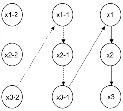
Example 1a is designed to show how to derive Granger causality from the
partial DAG of a TSCM in a simple case. The linear structural equation system of the TSCM in this example is as follows.
X1t = −0.2X3,t−1 +u1,t
X2t = −2X1,t+u2,t
X3t = −1.5X2,t+u3,t
where the residuals ui,t (i=1,2,3) are independent. An extended partial DAG of
the TSCM is given in Fig. 3. This extended partial DAG consists only of directed paths. Following Proposition 3.8 if there is a directed path from a lagged variable to another variable without going through any lagged variable of the latter, then the former variable Granger causes the latter. In this partial DAG we can read off many
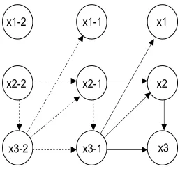
x1-2
x2-2
x3-2
x1-1
x2-1
x3-1
x1
x2
[image:12.612.234.361.336.451.2]x3
Figure 3: An extended partial DAG of the TSCM in Example 1a
directed paths. The pathX3,t−1 →X1,t does not go through lagged X1,t. Therefore
X3,t Granger causes X1,t. Similarly, the path X3,t−1 → X1,t → X2,t does not go
through laggedX2t. X3,talso Granger causes X2,t. The pathX2,t−1 →X3,t−1 →X1,t
does not pass through lagged X1,t. Hence,X2,t Granger causesX1,t. The only path
from X1,t−1 to X2,t: X1,t−1 → X2,t−1 → X3,t−1 → X1,t → X2,t−2 goes through
X2,t−1. Therefore X1,t does not Granger cause X2,t. For the same reason X1t does
not Granger cause X3,t, and X2t does not Granger cause X3,t either. The graphical
derivation result is given in the right graph in Fig. 4.
Multivariate Granger causality is the conditional dependence of one time series variable on another, given his own lagged variables as well as the rest lagged variables in the system. Following Proposition 3.9 if there is a directed path from a lagged variable to another variable in the partial DAG, then the former variable Granger causes the latter in multivariate setting. In the partial DAG of the TSCM, the
directed paths from a lagged variable to others are: X3,t−1 → X1,t and X3,t−1 →
Bivariaate Granger Causality in the TSCM
X1
X2
X3
Multivariate Granger Causality in the TSCM
X1
X2
X3
Figure 4: Granger Causality in Example 1a
X1,t and X2,t respectively. The graph for multivariate Granger causality is given in
the left graph in Fig. 4.
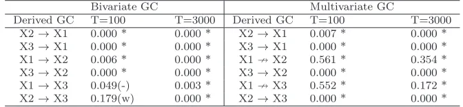
Bivariate GC Multivariate GC
Derived GC T=100 T=3000 Derived GC T=100 T=3000 X2→X1 0.002 * 0.000 * X29X1 0.590 * 0.105 *
X3→X1 0.001 * 0.000 * X3→X1 0.016 * 0.000 *
X19X2 0.614 * 0.466 * X19X2 0.473 * 0.706 *
X3→X2 0.362(w) 0.000 * X3→X2 0.014 * 0.000 *
X19X3 0.933 * 0.140 * X19X3 0.613 * 0.681 *
X29X3 0.549 * 0.731 * X29X3 0.321 * 0.118 *
Table 1: Bivariate and Multivariate Granger Causality Tests for Example 1a
We also run Granger causality tests in both bivariate and multivariate settings for data generated from the TSCM of Example 1a. The results are presented in Table 1. The left penal in Table 1 contain the test results of bivariate Granger causality. The right penal contains the test result for multivariate Granger causality. Among
12 small sample size cases (T = 100), there is only one case where the Granger
causality test result cannot confirm the derived Granger causality at 5% significance
level (See (w) in Table 1.). In large sample size cases (T = 3000), the test results
confirm all the derived Granger causality. (See * in Table 1.).
Example 1b differs from Example 1a only by adding an arrow X3,t−1 → X3,t
in the partial DAG. The linear structural equation system of the TSCM in this example is as follows.
X1,t = −0.2X3,t−1+u1,t
X2,t = −2X1,t+u2,t
X3,t = −1.5X2,t+ 0.5X3,t−1+u3,t
where the residuals ui,t (i=1,2,3) are independent. An extended partial DAG of
the TSCM is given in Fig. 5. The paths discussed in Example 1a are also present here. Therefore, the conditional dependencies remain: i.e. the bivariate Granger causality and the multivariate Granger causality derived in Example 1a hold also
in this example. In addition, through adding the arrow X3,t−1 → X3,t we have a
fork X1,t−1 ←X3,t−2 →X3,t−1 →X1,t →X2,t without crossing lagged X2,t−s. This
x1-2
x2-2
x3-2
x1-1
x2-1
x3-1
x1
x2
[image:14.612.234.362.24.143.2]x3
Figure 5: An Extended Partial DAG of the TSCM in Example 1b
Bivariaate Granger Causality in the TSCM
X1
X2
X3
Multivariate Granger Causality in the TSCM
X1
X2
[image:14.612.149.458.221.339.2]X3
Figure 6: Granger Causality in Example 1b
ofX3,t−2. Therefore,X1,t Granger causesX2,t. The graphical result for the bivariate
Granger causality is given in the left graph in Fig. 6.
For multivariate Granger causality the situation is the same as in Example 1a.
Therefore we have multivariate Granger causality: X3,t−1 Granger causes X1,t and
X2,t respectively. The Graph for multivariate Granger causality is given in the right
graph in Fig. 6.
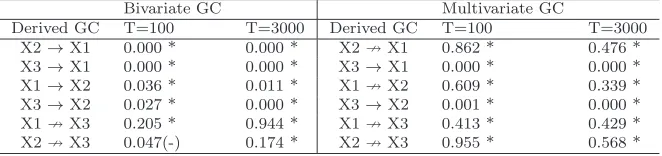
Bivariate GC Multivariate GC
Derived GC T=100 T=3000 Derived GC T=100 T=3000 X2→X1 0.000 * 0.000 * X29X1 0.862 * 0.476 *
X3→X1 0.000 * 0.000 * X3→X1 0.000 * 0.000 *
X1→X2 0.036 * 0.011 * X19X2 0.609 * 0.339 *
X3→X2 0.027 * 0.000 * X3→X2 0.001 * 0.000 *
X19X3 0.205 * 0.944 * X19X3 0.413 * 0.429 *
X29X3 0.047(-) 0.174 * X29X3 0.955 * 0.568 *
Table 2: Bivariate and Multivariate Granger Causality Tests for Example 1b
The results of the Granger causality tests in both bivariate and multivariate settings for data generated from the TSCM of Example 1b are presented in Table
2. Among 12 small sample size cases withT = 100, there is only one case where the
Granger causality test result rejects the null hypothesis suggested by the derived Granger causality at 5% significance level (See (-) in Table 2.). In large sample size
cases with T = 3000, the test results confirm the derived Granger causality (See *
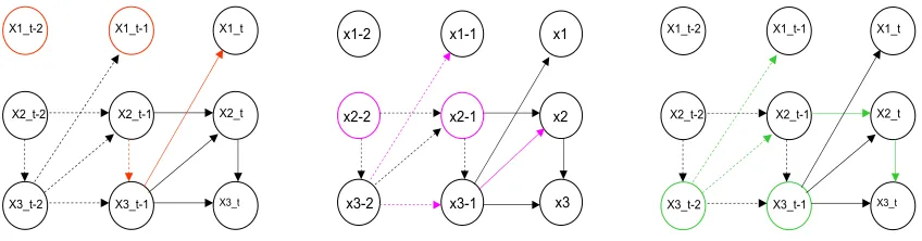
[image:14.612.133.464.506.584.2]Example 2 In the last example we see that a common cause at different lag lengths can lead to conditional dependence and henceforth the Granger causality relation. This simple example should show how the dependence due to a common cause can be blocked by lagged variables. The linear structural equation system of the TSCM in this example is as follows.
X1t = −0.2X3,t−1 +u1,t
X2t = −0.2X2,t−1 −0.2X3,t−1+u2,t
X3t = −1.5X2,t+ 0.5X3,t−1 +u3,t
where the residualsui,t (i=1,2,3) are independent. An extended partial DAG of the
TSCM is given in Fig. 7.
In this extended partial DAG, the two one-arrow paths: X3,t−1 → X1,t and
X3,t−1 → X2,t imply X3t Ganger causes X1,t and X2,t. The two two-arrows paths:
X2,t−1 → X3,t−1 → X1,t and X2,t−1 → X2,t → X3,t imply X2,t Granger causes X1,t
and X3,t.
x1-2
x2-2
x3-2
x1-1
x2-1
x3-1
x1
x2
[image:15.612.233.362.261.384.2]x3
Figure 7: Partial DAG of TSCM in Example 2
Since no arrow goes fromX1,t,X1,t can only Granger cause others via conditional
dependence duo to some common causes. The forkX1,t−1 ←X3,t−2 →X3,t−1 →X2,t
does not cross lagged X2,t. Therefore X1,t Granger cause X2,t. The fork X1,t−1 ←
X3,t−2 ← X2,t−2 → X2,t−1 → X2,t → X3,t crosses lagged X3,t at X3,t−2. Therefore
this fork does not imply Granger casuality of X1t for X3,t. Further, because any
path ending at X1,t−j, must go through X3,t−j, i.e. X3,t−j blocks the dependence
betweenX1,t−j andX3,t. In other word conditional on laggedX3,t−j,X1,t−j andX3,t
becomes independent. Therefore X1,t does not Granger cause X3,t. This graphical
derivation of the bivariate Granger causality is shown in detail in Fig. 8.
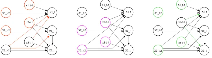
For multivariate Granger causality, we look at the three partial DAGs in Fig. 9. In the partial DAG on the left side the orange nodes are the conditioning set.
The orange paths do not go through the orange nodes, which implies that X3,t
Granger causes X1,t and X2,t. In the partial DAG in the middle of Fig. 9 the
pink nodes represent the conditioning set. There is no directed path from a lagged
X1,t into X2,t orX3,t. Therefore X1,t does not Granger cause X2,t and X3,t. In the
partial DAG on the right side of Fig. 9, the green nodes are the conditioning set.
The green path from X2,t−1 to X3,t does not go through the green nodes, which
implies X2,t Granger causes X3,t. The results of the graphical analysis of bivariate
X1_t-1
X2_t-1
X3_t-1
X1_t
X2_t
X3_t X1_t-2
X2_t-2
X3_t-2
x1-2
x2-2
x3-2
x1-1
x2-1
x3-1
x1
x2
x3
X1_t-1
X2_t-1
X3_t-1
X1_t
X2_t
X3_t X1_t-2
X2_t-2
X3_t-2
In the left extended partial DAG, the orange nodes represent the laggedX1,t, the orange
pathsX3,t−1→X1,t andX2,t−1 →X3,t−1→X1,t do not cross the orange nodes, implying
that X2,t and X3,t Granger cause X1,t respectively. In the middle graph the pink nodes
represent the lagged X2,t. The directed path X3,t−1 → X2,t and the fork X1,t−1 ←
X3,t−2 → X3,t−1 → X2,t do not cross the pink nodes, implying X1,t and X3,t Granger
causeX2,t respectively. In the right graph, the green pathX2,t−1 →X2,t→X3,t does not
cross the green nodes. This implies X2,t Granger causes X3,t. The green fork X1,t−1 ←
X3,t−2 → X2,t−1 → X2,t → X3,t crosses X3,t−2. It does not imply X1,t Granger causes
[image:16.612.86.510.19.130.2]X3,t.
Figure 8: Bivariate Granger Causality in Example 2
Bivariate GC Multivariate GC
Derived GC T=100 T=3000 Derived GC T=100 T=3000 X2→X1 0.000 * 0.000 * X29X1 0.890 * 0.221 *
X3→X1 0.000 * 0.000 * X3→X1 0.001 * 0.000 *
X1→X2 0.474(w) 0.000 * X19X2 0.132 * 0.363 *
X3→X2 0.005 * 0.000 * X3→X2 0.004 * 0.000 *
X19X3 0.315 * 0.259 * X19X3 0.247 * 0.453 *
X2→X3 0.045 * 0.000 * X2→X3 0.038 * 0.000 *
Table 3: Bivariate and Multivariate Granger Causality Tests for Example 2
[image:16.612.132.465.308.386.2]X1_t-1
X2_t-1
X3_t-1
X1_t
X2_t
X3_t
X1_t-1
X2_t-1
X3_t-1
X1_t
X2_t
X3_t
X1_t-1
X2_t-1
X3_t-1
X1_t
X2_t
X3_t
In the left partial DAG, the orange path X3,t−1 →X1,t does not cross the orange nodes.
This implies X3,t Granger causes X1,t. In the middle graph there is no path from X1,t−1. So,X1,t causes neitherX2,t norX3,t. In the right graph, the green pathX2,t−1 →X2,t →
[image:17.612.154.447.18.130.2]X3,t does not cross the green nodes. This impliesX2,t Granger causesX3,t.
Figure 9: Multivariate Granger Causality in Example 2
Bivariaate Granger Causality in the TSCM
X1
X2
X3
Multivariate Granger Causality in the TSCM
X1 X2
X3
Figure 10: Graphs for Granger Causality in Example 2
Example 3is an example withN = 3 andp= 2. The linear structural equation
system of the TSCM is given as follows.
X1t = 0.5X1,t−1−0.4X2,t−1+ 0.3X3,t−1+ 0.35X1,t−2−0.12X3,t−2+u1,t
X2t = 0.5X2,t−1+ 0.35X2,t−2+ 0.23X3,t−2+u2,t
X3t = −1.5X2,t−0.2X2,t−1+ 0.5X3,t−1+ 0.35X3,t−2+u3,t
where the residuals ui,t (i=1,2,3) are independent. The partial DAG of the TSCM
is given in Fig. 11.
An extended partial DAG is given in in Fig.12. In order to investigate the bivariate Granger causality in this TSCM, we first look at the nodes in orange
color representing lagged variables ofX1,t and orange paths ending at X1,t without
crossing the orange nodes. The starting points of the paths are X2,t−1 and X3,t−1
respectively. These two paths imply X3,t Granger causes X1,t, and X2,t Granger
causes X1,t. Next, we look at the pink nodes representing the lagged variables of
X2,t and pink paths ending atX2,t. The pink directed path X3,t−2 →X2,t and the
pink fork X1,t−1 ← X3,t−2 → X2,t do not cross the pink nodes. Therefore we have
X1,t Granger causesX2t; andX3,t Granger causesX2,t. At last we look at the green
nodes representing the lagged variables of X3,t and the green paths ending at X3,t.
X1_t-2
X2_t-2
X3_t-2
X1_t-1
x2-t-1
x3-t-1
X1_t
X2_t
[image:18.612.241.356.30.142.2]X3_t
Figure 11: Partial DAG of TSCM in Example 3
not cross the green nodes. Therefore X1,t Granger causes X3,t, and X2,t Granger
causesX3,t.
x1-2
x2-2
x3-2
x1-1
x2-1
x3-1
x1
x2
x3 x1-3
x2-3
[image:18.612.208.361.250.375.2]x3-3
Figure 12: Bivariate Granger Causality in Example 3
For multivariate Granger causality the conditional set includes all other lagged variables. We look first at the partial DAG at the right side in Fig. 13. The orange
nodes represent lagged X1,t and lagged X2,t. The orange paths: X3,t−1 →X1,t and
X3,t−2 →X2,t imply theX3,t Granger causesX1,t and it also Granger causesX2,t. In
the middle graph in Fig. 13 we see the partial DAG with some pink nodes presenting
lagged variables ofX2,t and lagged variables ofX3,t. No paths ending at X2,t orX3,t
will not cross the pink nodes. ThereforeX1,t will not Granger causeX2,t and it will
not Granger cause X3,t either. In the right partial DAG in Fig.13 we have green
nodes representing lagged variables of X1,t and lagged variables of x3,t. We have
two directed pathsX2,t−1 →X1,t and X2,t−1 →X3,t. Both of them do not cross the
green nodes. This implies thatX2,t Granger causes X3,t and it also Granger causes
X1,t.
Bivariate GC Multivariate GC
Derived GC T=100 T=3000 Derived GC T=100 T=3000 X2→X1 0.000 * 0.000 * X2→X1 0.007 * 0.000 *
X3→X1 0.000 * 0.000 * X3→X1 0.000 * 0.000 *
X1→X2 0.006 * 0.000 * X19X2 0.561 * 0.354 *
X3→X2 0.000 * 0.000 * X3→X2 0.000 * 0.000 *
X1→X3 0.049(-) 0.003 * X19X3 0.552 * 0.172 *
X2→X3 0.179(w) 0.000 * X2→X3 0.000 * 0.000 *
[image:18.612.129.465.622.700.2]X1_t-2
X2_t-2
X3_t-2
X1_t-1
x2-t-1
x3-t-1
X1_t
X2_t
X3_t
X1_t-2
X2_t-2
X3_t-2
X1_t-1
x2-t-1
x3-t-1
X1_t
X2_t
X3_t
X1_t-2
X2_t-2
X3_t-2
X1_t-1
x2-t-1
x3-t-1
X1_t
X2_t
[image:19.612.104.466.23.123.2]X3_t
Figure 13: Multivariate Granger Causality in Example 3
The graphically derived results for the bivariate and the multivariate Granger causality are presented in Fig. 14.
Bivariaate Granger Causality in the TSCM
X1
X2
X3
Multivariate Granger Causality in the TSCM
X1 X2
X3
Figure 14: Granger Causality in Example 3
The the Granger causality test results using the data generated from the TSCM in Example 3 are presented in Table 4. For a sample size of 100, there are two cases in which the Granger causality tests cannot confirm the derived Granger causality at 5% significance level (See (w) and (-)in Table 4.). For a sample size of 3000 the tests confirm all the derived Granger causality between the time series.
These 4 examples show that it is quit easy to derive the bivariate Granger causal-ity and the multivariate Granger causalcausal-ity for the time series in a TSCM. However, when the number of involved time series is large and the topology of partial DAGs is complicated, it can be a messy task to derive the Granger causality graphs from the partial DAGs by hand. We have implemented a computer program to transform a partial DAG into the Granger causality graphs for both bivariate and multivariate cases using Propositions 3.8 and 3.9.
5
Looking Behind Granger Causality between Wages
and Prices
Wage-price spiral is a concept in macroeconomics that deals with the causes and effects of inflation. The wage-price spiral hypothesis suggests that rising wages increase income, thus increasing the demand for goods and causing prices to rise. Rising prices cause demand for higher wages, and leading to higher production costs
and further upward pressure on prices12. A bivariate Granger-causality test for the
two time series dpt - the price inflation and dwt - the wage inflation of Australian
data show that dpt and dwt are mutually Granger cause to each other (See Table
5). This result seems to support the wage price spiral hypothesis. However, as we
F-test P-value DW → DP 3.2249119 0.01520841
DP → DW 2.9290993 0.02406271
Table 5: Bivariate Granger Causality Tests for Price and Wage
have seen in the previous section, a mutual Granger causality between two time series does not necessarily imply that they are cause to each other. In order to give a causal explanation to this mutual Granger causality, we need to take relevant variables that may potentially influence the wage inflation and the price inflation into account. For this purpose we adopt the theoretical framework as set out in Flaschel and Krolzig (2003) as well as in Chen and Flaschel (2006), in which two Phillips curves, one for price inflation and one for wage inflation are used to describe the dynamic wage-price spiral. The theoretical formulation of the Phillips curves are as follows.
dw = βw1(Vl−V¯l) +κwdp+ (1−κw)πm+βw2dz (5.5)
dp = βp1(Vc−V¯c) +κpdw+ (1−κp)πm+βp2dz (5.6)
In these symmetrically formulated two Phillips curve equations, we consider both push and pull factors representing demand pressure and cost pressure respectively. Both wages and prices react to their own measure of demand pressure: namely
Vl−V¯l andVc−V¯c, in the market for labor and for goods, respectively. We denote
byVlthe rate of labour utilization on the labor market and by ¯Vlthe NAIRU-level of
this rate, and similarly byVc the rate of capacity utilization of the capital stock and
¯
Vcthe normal rate of capacity utilization of firms. These demand pressures are both
augmented by a weighted average of cost-pressure terms: cost pressure perceived by
workers is a weighted average of the currently evolving rate of price inflationdpand
the expected price inflation,πm. Similarly, cost pressure perceived by firms is given
by a weighted average of the currently evolving rate of wage inflation,dw and again
the measure of expected inflation. Further the Phillips curves are augmented by
changes of labor productivity dz that impacts positively on the wage inflation and
negatively on the price inflation (see Flaschel and Krolzig (2003) for more details of theoretical arguments on this type of two Phillips curves.)
The empirical data for the relevant variables are taken from Australian Bureau
of Statistics13. The data shown below are quarterly, seasonally adjusted, annualized
12
See http://www.investorwords.com/5850/wage price spiral.html
13
where necessary. The data used in this investigation are from 1978:3 to 2009:2, which correspond to the longest commonly available time series for the set of variables used in the investigation.
Variable Transformation Description
e 100−U RAT E URATE: Unemployment Rate(%)
e: Employment Rates
u GDP H P trendGDP 100 GDP: Real Gross Domestic Product
Chain volume measures.
DGP HPtrend: the trend component of HP filter applied to GDP.
u: Capacity utilization rate, ratio
dw AW E−AW E(−1)
AW E(−1) 400 AWE: Average Weekly Earnings,
dw: wage inflation, annualized
dp CP I−CP I(−1)
CP I(−1) 400 CPI: Consumer price index, all groups, Index 1990 = 100
dp: price inflation, annualized
z H OU RSGDP HOURS: Total (Actual hours worked)
z: labor productivity
dz z−z(−1)
z(−1) 400 dz: change of labor productivity, annualized
πm
[image:21.612.139.459.90.353.2]: CIE Consumer inflation expectation (%), survey data, Westpac-Melbourne Institute Consumer Survey.
Table 6: Raw data used for empirical investigation of the wage-price spiral
We construct a TSCM consisting of six time series variables (dp, dw, πm, e, u, dz)14.
Through a series of unit root testsdp, dw, πm, e, u, dz are confirmed to be stationary,
where the unit test for πm is run after controlling for a structural break in 1991:2.
To obtain an estimated TSCM, we apply the method of inferred causation as described in Chen (2010). Concretely obtaining the estimated TSCM for the 6 time series consists of the following steps:
• Choose a reasonable ˆp
• Estimate the covariance matrix ˆΣ for (Xt, Xt−1, ..., Xt−pˆ)
• ApplyP C algorithm15 to ˆΣ to obtain a DAG for (X
t, Xt−1, ..., Xt−pˆ)
• Delete all arrows that do not end atXtto obtain a partial DAG for the TSCM.
If there are no arrows starting at some nodes in Xt−pˆ, then the choice of ˆpis
large enough. Otherwise GOTO the first step and increase ˆpby one.
• Apply greedy search algorithm with the partial DAG from the P C algorithm
as a starting partial DAG to obtain the final partial DAG.
14
We correct the data of dpwith a dummy variabled GST, to take into account of the impact of the introduction of the good and service tax (GST) on prices in the third quarter 2000.
15
The resulting partial DAG for the six time series is given in Fig. 15. The linear structural equations of this TSCM are:
dpt= 0.76
14.69π
m
t + 0.52
3.50ut−3−53−3..0361 +ǫpt (5.7)
dwt= 0
8.34.72π
m
t−1 + 0.48
2.59et+ 03..2194dzt−1 −45−2..2863 +ǫwt (5.8)
πtm = 0.96
40.92π
m
t−1+ 0.23
−1.18+ǫπ
mt (5.9)
et=−0.08
−4.57
ut−3−0.36
−9.81et−3+ 138.35.13et−1+ 95..0672 +ǫet (5.10)
ut=−0.67
−6.88et−2 + 07..7200et+ 014.73.17ut−1+ 03..0383dzt−224..9541+ǫut (5.11)
dzt=−0.40
−4.81
dzt−1+ 2.23
4.3 +ǫzt. (5.12)
[image:22.612.110.502.71.449.2]dp-4 dw-4 S-4 e-4 u-4 dz-4 dp-3 dw-3 S-3 e-3 u-3 dz-3 dp-2 dw-2 S-2 e-2 u-2 dz-2 dp-1 dw-1 S-1 e-1 u-1 dz-1 dp dw S e u dz
Figure 15: Partial DAG of the Wage Price Spiral
The partial DAG says thatdptis influenced byπtmandut−3; anddwtis influenced
by πtm−1, et and dzt−1. But dpt, dwt and their lags don’t influence other variables:
dzt, πtm, et and ut. In other words the latter four variables are determinants of the
price inflation and wage inflation. This confirms that our choices of variables are reasonable.
Importantly, the two Phillips curve equations confirm largely the theoretical formulation as given in (5.6) and (5.5), albeit some variables are statistically in-significant: the price inflation and the wage inflation are driven by the common cost
pressure variable πm
t at different lags, both direct cost pressure dwt and dpt have
no significant influence on the price inflation and the wage inflation respectively. A
labour productivity increasedztwill impact positively on the wage inflation with one
lag, but has no impact on the price inflation. The market specific demand pressure
etfor the wage inflation andut−3 for the price inflation have significant influence on
dwt and dpt respectively.
(See Fig. 18). Indeed the estimated TSCM implies the mutual bivariate Granger causality between the wage inflation and the price inflation. However, the TSCM supports neither the hypothesis that the wage inflation causes the price inflation nor the hypothesis that the price inflation causes the wage inflation. Because no
arrows start from lagged dpt or lagged dwt in the partial DAG of the estimated
TSCM, there is no directed paths from a node of laggeddpttodwt or from a lagged
dwt to dpt. The mutual bivariate Granger causality between the wage inflation and
[image:23.612.108.496.136.280.2]dp_t-4 dw_t-4 _t-4 e_t-4 u_t-4 dz_t-4 dp_t-3 dw_t-3 _t-3 e-3 u_t-3 dz_t-3 dp_t-2 dw_t-2 _t-2 e-2 u_t-2 dz_t-2 dp_t-1 dw_t-1 _t-1 e-1 u_t-1 dz_t-1 dp_t dw_t _t e u_t dz_t dp_t-4 dw_t-4 _t-4 e_t-4 u_t-4 dz_t-4 dp_t-3 dw_t-3 _t-3 e-3 u_t-3 dz_t-3 dp_t-2 dw_t-2 _t-2 e-2 u_t-2 dz_t-2 dp_t-1 dw_t-1 _t-1 e-1 u_t-1 dz_t-1 dp_t dw_t _t e u_t dz_t dp_t-6 dw_t-6 _t-6 e_t-6 u_t-6 dz_t-6 dp_t-5 dw_t-5 _t-5 e_t-5 u_t-5 dz_t-5
Figure 16: Common Cause Processes in the TSCM for the Wage Price Spiral
the price inflation is an effect of common cause processes: the inflation expectation, the labour utilization rate and the capacity utilization rate as well as the labour productivity growth. Now we look at the common cause processes in detail. On the
left graph of Fig. 16 we see a fork in orange color from dwt−1 to dpt and a fork in
pink color fromdpt−1 todwt. These two forks imply that the common cause process
πt leads to the mutual Granger causality between dwt and dpt. These two forks
consist of directed paths from laggedπt to dwt and dpt respectively, implying that
πt Granger causes dwt and dpt respectively. On the right graph in Fig. 16 we see
also a fork in orange color fromdwt−1 to dpt and a fork in pink color fromdpt−1 to
dwt. These two forks imply that the common cause processetis a further reason for
the mutual Granger causality between dwt and dpt. The two forks starting at et−5
and et−6 respectively imply that et Granger causes dwt and dpt.
Beside πt and et, ut and dzt are also common cause processes that lead to the
mutual Granger causality between dwt and dpt. On the left graph in Fig. 17 we see
a fork in pink color fromdwt−1 todpt and a fork in orange color from dpt−1 todwt.
The starting nodes of the two forks are ut−4 and ut−3 respectively, meaning thatut
is a common cause process that leads to the mutual Granger causality betweendwt
and dpt. Further the two forks consist of directed paths from lagged ut to dwt and
dpt, implying thatut Granger causes dwt and dpt.
On the right graph of Fig. 17 we see also a fork in orange color from dwt−1 to
dptand a fork in pink color fromdpt−1 todwtwith starting nodes atdzt−3 anddzt−4
respectively. Therefore, dzt is also a common cause process and dzt Ganger causes
dpt and dwt, respectively.
dp_t-4 dw_t-4 _t-4 e_t-4 u_t-4 dz_t-4 dp_t-3 dw_t-3 _t-3 e-3 u_t-3 dz_t-3 dp_t-2 dw_t-2 _t-2 e-2 u_t-2 dz_t-2 dp_t-1 dw_t-1 _t-1 e-1 u_t-1 dz_t-1 dp_t dw_t _t e u_t dz_t dp_t-4 dw_t-4 _t-4 e_t-4 u_t-4 dz_t-4 dp_t-3 dw_t-3 _t-3 e-3 u_t-3 dz_t-3 dp_t-2 dw_t-2 _t-2 e-2 u_t-2 dz_t-2 dp_t-1 dw_t-1 _t-1 e-1 u_t-1 dz_t-1 dp_t dw_t _t e u_t dz_t
Figure 17: Common Cause Processes in the TSCM for the Wage Price Spiral
run tests for the 30 possible pairs of the six time series. At 5% significance level, in 22 out of 30 cases, the empirical test results confirm the derived Granger causality from the TSCM. In 6 cases the p-values of the tests are not under 5% to support the derived Granger causality (See (w) in Table 7.). Only in two cases the empirical test results would reject the null hypotheses suggested by the the derived Granger causality (See (-) in Table 7.). In the multivariate setting we also run tests for all 30 possible pairs of time series in the TSCM and show the results in Table 8. In 21 out of 30 cases the empirical test results confirm the derived Granger casuality at 5% significance level. In 5 cases the the p-values of the tests are over 5% and in four cases, the empirical test rejects the null hypothesis suggested by the derived Granger causality.
Taking into account of the sample uncertainty, the strength of the conditional de-pendence embodied in the TSCM and the limited sample size, the empirical Granger causality tests confirm very well the derived Granger causality from the estimated TSCM. We conclude that the TSCM indeed provides a causal explanation to the Granger causality relation in both bivariate and multivariate settings.
Bivariaate Granger Causality in the TSCM of the W−P Spiral
dp dw pi e u dz
Multivariate Granger Causality in the Wage Price Spiral
dp dw
pi
e
[image:24.612.127.234.511.653.2]u dz
Variable Derived GC Variable F-test P-value DW → DP 3.2249119 1.520841e-02*
PI → DP 7.0207238 4.516021e-05*
E → DP 2.4660186 4.910483e-02*
U → DP 2.2202503 7.140512e-02(w)
DZ → DP 0.3802965 8.223070e-01(w)
DP → DW 2.9290993 2.406271e-02*
PI → DW 3.6770926 7.527255e-03*
E → DW 2.772306 3.066234e-02*
U → DW 2.692449 3.468061e-02*
DZ → DW 5.1477921 7.706622e-04*
DP 9 PI 0.7644344 5.506152e-01*
DW 9 PI 0.4417655 7.781739e-01*
E 9 PI 4.9946669 -9.76E-04(-)
U 9 PI 0.8331082 5.069403e-01*
DZ 9 PI 1.3854465 2.436745e-01*
DP → E 1.1291627 3.465610e-01(w)
DW → E 1.7219652 1.502268e-01(w)
PI 9 E 1.8088241 1.322161e-01*
U → E 6.6080615 8.369460e-05*
DZ → E 0.4391116 7.800984e-01(w)
DP 9 U 0.2984294 8.784242e-01*
DW → U 1.8468289 1.249931e-01(w)
PI 9 U 4.5508841 -1.94E-03(-)
E 9 U 4.2266619 3.202243e-03*
DZ → U 2.7196207 3.325832e-02*
DP 9 DZ 0.4706951 7.571350e-01*
DW 9 DZ 0.2354697 9.178189e-01*
PI 9 DZ 0.430392 7.864128e-01*
E 9 DZ 1.1891048 3.196607e-01*
[image:25.612.166.425.33.332.2]U 9 DZ 1.4471262 2.233463e-01*
Table 7: Bivariate Granger Causality Tests
Variable Derived GC Variable F-test P-value DW 9 DP 0.760995 0.5185486 *
PI → DP 8.07E+00 7.14E-05 *
E 9 DP 0.3179057 0.8124003 *
U → DP 1.8425941 0.1442317 (w)
DZ 9 DP 0.2368921 0.870454 *
DP 9 DW 2.45067119 0.06782165 *
PI → DW 1.5683837 0.2017113 (w)
E → DW 1.0643224 0.3677551 (w)
U → DW 0.2935767 0.8299544 (w)
DZ → DW 8.56E+00 4.07E-05 *
DP 9 PI 0.750059 0.5248087 *
DW 9 PI 0.5351803 0.6592183 *
E 9 PI 3.83289689 0.01203739 (-)
U 9 PI 0.4889514 0.6907254 *
DZ 9 PI 0.9986012 0.3967798 *
DP 9 E 0.3763536 0.7702406 *
DW 9 E 1.1493437 0.3330056 *
PI 9 E 0.8835073 0.4523915 *
U → E 5.588050119 0.001378957 *
DZ → E 1.41724 0.2421553 *
DP 9 U 0.8644279 0.4622166 *
DW 9 U 1.2576007 0.2930603 *
PI → U 5.86275954 0.00098738 (-)
E → U 3.54723908 0.01719812 *
DZ → U 0.3144241 0.8149147 (w)
DP 9 DZ 0.2826493 0.8378182 *
DW 9 DZ 0.3663855 0.7774112 *
PI 9 DZ 0.7670196 0.5151247 *
E 9 DZ 3.55643613 0.01700151 (-)
U 9 DZ 3.34860888 0.02204906 (-)
[image:25.612.162.426.389.687.2]6
Concluding Remarks
In this paper we present a graph-theoretic causal approach to investigate the causal structure behind the conditional dependence revealed by Granger causality tests. We summarize the main results of this approach. Under quit mild assumptions on the time series: the temporal causal order constraint, the time invariant causal structure constraint and the time limited causal constraint, a time series causal model can
be represented by a partial DAG. Based on d −separation and d −connection
criteria we develop simple rules to create directed graphs for bivariate as well as multivariate Granger causalities from the underlying partial DAG of a TSCM. While the directed graphs for Granger causality provide a visual, concise and informative way to communicate the pairwise Granger-causal and nonGranger-causal relations among time series, the partial DAG visualizes the complex causal structure among the relevant time series behind the Granger causality relation.
For a given set of time series data of interest, on the one hand, Granger causality tests can be implemented to provide evidence of Granger causality among the time series. One the other hand, a TSCM can be constructed and the Granger causality graphs can be derived based on the estimated partial DAG of the TSCM obtained through the learning algorithm as demonstrated in the paper. Contrasting the results of the Granger causality tests with the derived Granger casuality graphs, we are able to look behind the Granger causality relation and provide a causal explanation to the conditional dependence manifested in the results of the Granger causality tests.
Our investigation on the wage price spiral in the Australian economy supports neither the hypothesis that the wage inflation causes the price inflation nor that the price inflation causes the wage inflation. By contrast, it shows that the bivariate Granger causality between the wage inflation and the price inflation is caused by common cause processes: the inflation expectation, the labour utilization rate and the capacity utilization as well as the labour productivity growth.
The analytic procedure in this paper is to a large extent data-driven: the Granger causality tests, the inference of the partial DAG and the derivation of Granger causality graphs. Consequently, the output results depend solely on the chosen input data. It is, therefore, crucial to select carefully the relevant time series variables for a TSCM in order to obtain a useful result. Since the selection of relevant variables is so critical to the output results, it calls for an operational criterion to evaluate
the soundness of the selection. In the setting of independent data, output of P C
algorithm provides indications of missing cofounders16. Exploring the applicability
of P C algorithm in detecting presence of missing causal processes in a TSCM is
a worthwhile future research issue, which would add important credibility to the method presented in this paper.
16
References
Chen, P. (2010). A time series causal model. Working paper, mimeo Melbourne University.
Chen, P. and Flaschel, P. (2006). Measuring the interaction of wage and
price Phillips curves for the U.S. economy. Studies in Nonlinear Dynamics and
Econometrics, 10, No. 4:Article 2.
Chen, P. and Hsiao, C. (2007). Learning causal relations in multivariate time
sereis data. Economics: The Open-Access, Open-Accessment E-Journal, 1,
2007-11.
Eichler, M. (2007). Granger causality and path diagrams for multivariate time
series. Journal of Econometrics, 137:334–353.
Flaschel, P. and Krolzig, H. (2003). Wage and price Phillips curves. An
em-pirical analysis of destabilizing wage-price spirals. Center of Empirical
Macroeco-nomics, Bielefeld University.
Granger, C. W. J. (1980). Testing for causality: A personal viewpoint. Journal of Economic Dynamics and Control, 2:329–352.
Hendry, D.(1995). Dynamic Econometrics. Oxfort University Press, 1st edition.
Hoover, K. (2005). Automatic inference of the contemporaneous causal order of
a system of equations. Econometric Theory, 21:69–77.
— (2008). Causality in economics and econometrics. The New Palgrave Dictionary
of Economics Online, Second Edition. Steven N. Durlauf and Lawrence E. Blume Eds. Palgrave Macmillan.
— (2010). Economic theory and causal inference. in HANDBOOK OF THE
PHILOSPHY OF ECONOMICS, Uskali M¨aki, ed., Forthcoming.
Kalisch, M. and Buehlmann, P.(2007). Estimating high-dimensional directed
acyclic graphs with the pc-algorithm. Journal of Machine Learning Research,
8:613–636.
Pearl, J.(2000). Causality. Cambridge University Press, 1st edition.
Pearl, J. and Verma, T.(1991). A theory of inferred causation. In J.A. Allen, R. Fikes, and E. Sandewall(Eds.), Principles of Knowledge Representation and Rea- soning: Procedings of the 2nd International Conference, San Mateo, CA: Morgan Kaufmann, pages 441–452.
Reichenbach, H. (1956). The Direction of Time. Berkeley, University of Los Angles Press.
Robins, J., Scheines, R., Sprites, P., and Wasserman, L. (2003). Uniform
Spirtes, P., Glymour, C., and Scheines, R. (2000). Causation, Prediction and Search. Springer-Verlag, New York / Berlin / London / Heidelberg / Paris, 2nd edition.