Munich Personal RePEc Archive
Productive Public Expenditure and Debt
Dynamics: a Theoretical Framework
based on Intertemporal Optimization
Bhatt Hakhu, Antra
Tata Institute of Social Sciences
9 December 2010
1
Productive Public Expenditure and Debt Dynamics: a Theoretical Framework based
on Intertemporal Optimization
Dr. Antra Bhatt Hakhu1
Centre for Research and Development Tata Institute of Social Sciences, Mumbai, India
[email protected] , [email protected],
JEL Classification: H63, E62, C61
Key words: Public Debt, Sustainability, Public Expenditure, Dynamic Optimization
1
2
Abstract
The paper aims to explore the dynamics between components of public expenditure and debt using an intertemporal optimization framework. Public expenditure is classified as
productive and ‘less-productive’ based on the rationale that an increase in the share of productive expenditure in total public expenditure (phi) affects public debt inversely in the
long-run. The ‘second-order’ conditions resulting from the model demonstrate that when
phi is less than or equal to half, an inverse relationship between phi and public debt will
hold only if private investment stimulus is high in the economy. Beyond its optimal level, an increase in phi could still affect public debt inversely; however, this will be at the cost of ‘crowding out’ of private investment. To understand whether phi is the share of capital
3
1. Introduction
Public debt sustainability is vital for both industrialized and emerging market countries. However, in emerging economies, the painful economic adjustments associated with a financial crisis that are aggravated by an unstable access to capital markets are an important incentive to keep public debt within sustainable grounds. One of the important methods to tackle this issue is to maintain fiscal balances in a way to offset the impact of transitory factors, thereby, preventing public debt from getting on to a divergent path. There is an abundance of literature on this issue, where tax based fiscal consolidation and its role in curtailing public debt is discussed. Furthermore, recent revival of interest in growth theory has led to deeper research on the link between public expenditure, growth and public debt (Alesina and Perotti 1999; Blanchard and Perotti, 1999; Giuliodori and Beetsma, 2004; Romer and Romer, 2007; Caldara and Kamps, 2008; Barrios, Langedijk and Pench 2010).
More specifically, on the issue of expenditure based fiscal consolidation, Devarajan, Swaroop, Zou (1996) made a seminal contribution through their paper where they established a direct relationship between productive2 components of public expenditure and growth. Based on a dynamic optimization framework, they demonstrated that until the
level of ‘optimal’ productive expenditure is reached in the economy, it is worthwhile to increase the level of productive type expenditures in the economy. A number of other empirical studies that analyzed the relationship between components of public expenditure and debt, as discussed in the forthcoming section, followed. However, as far as the author’s knowledge goes, few attempts have been made to understand the direct link between components of public expenditure and debt so far.
This paper attempts to add to the existing body of literature by examining the relationship between components of public expenditure and sovereign debt in an inter-temporal optimization framework. The aim of this theoretical exploration is to understand the dynamics of productive public expenditure with the level of public debt in light of the
4
consumption and investment choices of the representative agent in the economy. To complement the theoretical analysis and to test the implications of the model, an empirical exercise using Indian public finance data is performed. The key objective of the empirical analysis is to identify the productive components of public expenditure and to understand how they affect debt dynamics using stationarity, cointegration and ECM modelling techniques in the context of a developing and emerging economy like India.
The remainder of the paper is organized as follows. Section 2 summarizes the extant theoretical and empirical literature on public expenditure, private investment, growth and debt. Section 3 presents the theoretical framework that has been formulated in the paper by discussing the assumptions of the model, variables used, methodology, setting up of the framework, first and second order conditions followed by the implications. Section 4 deals with the empirical analysis of Indian Public Finance data. This part of the paper focuses on the reasons for choosing Indian data, the specific objectives of the empirical analysis, data sources, methodology, analysis and the key findings. Section 5 summarizes the key implications of the theoretical model and the key findings of the empirical analysis to discuss the issue at hand and to draw policy implications from the analysis.
2. Previous Research: Public Expenditure, Growth and Debt
5
2.1 Theoretical Underpinnings
Arrow and Kurz (1970) in their seminal paper developed a model where consumers derive utility from private consumption as well as public capital stock. The literature on endogenous growth theories has further generated models linking public spending with the economy's long-term growth rate. Barro (1990, 1991) introduce government expenditure and classify public spending as consumption and investment expenditure. The empirical findings suggest that all non productive expenditures can have a negative effect on the growth rate of real GDP per capita in the long term. This would lead to higher level of debt
as the growth rate will be reduced. However, in Barro’s models public spending only
affects the economy's transitional growth rate, while the steady-state growth rate remains unaltered. Devarajan, Swaroop, Zou (1996) relax the assumption of exogenous public spending. They build an optimization problem with two types of expenditure, productive and unproductive. They find that there is an optimal level of productive expenditure in an economy, beyond which such expenditures can have a negative impact on growth, due to over investment in capital and diminishing returns to scale. Agenor and Neanidis (2006) explored a similar framework years later. They analyzed the possible optimal allocation of public spending among health, education and infrastructure, taking into account the dynamics between the sectors.
The theoretical work of Chatterjee and Turnovsky (2005, 2007) was also an important contribution as they use an open economy model to analyze the effect of financing public investment through foreign aid. Their results show that an important determinant of the impact on growth is linked to whether the foreign aid is used for investment purposes or not. In their recent work, Christie, Rioja (2012) are able to demonstrate that fiscal conditions of the economy are a key determinant of the optimal strategy to finance public investment. Thus, lending support to the fact that public investment must be increased only
6 2.2 Extant Empirical Literature
Carranza, Daude, Melguizo (2014) look at the relationship between fiscal consolidation and public investment in six of the main Latin American economies namely Argentina, Brazil, Chile, Colombia, Mexico, and Peru. They find that simple austerity measures that focus on cuts in current expenditures may not be appropriate for fiscal consolidation. They point to the case of Peru where fiscal imbalances were reduced by means of measures that favoured public infrastructure investment and placed ceilings solely on current expenditures. Gupta, Kangur et. al (2014) look at the effect of public investment on capital
accumulation and growth. Based on an empirical analysis performed on a panel of low-income economies, they find that the quality of public investment is statistically significant in explaining variations in economic growth. Panizza, Presbitero (2014) use a panel of OECD countries to look at the links between economic growth and public debt along with examining a causal relationship between them. Their results are consistent with other studies where a negative correlation between the two variables is found. However, studies such as Herndon, Ash and Pollin (2014) do not find such a causal relationship while analyzing the data for the same set of countries for a similar time period even if the negative correlation exists. Thus, recent empirical literature has clearly shown that sovereign capital expenditure could boost economic growth and hence affect public debt inversely, in the long run.
7
growth. They replicate the technique used by Reinhart and Rogoff (2010A and 2010B) to analyze the effect of high public debt/GDP on the growth of an economy. Using a dataset of advanced economies they find that high public debt/GDP ratios do not necessarily reduce a country’s GDP growth. Thus, the relationship between economic growth and debt could be stronger for developing countries in comparison to that of their advanced counterparts.
Bose, Haque, Osborne (2003) examined the growth effects of government expenditure for a panel of 30 developing economies with a focus on sectoral expenditures during the 1970s and 80s. Their main empirical result is that the ratio of government capital expenditure to GDP is positively and significantly correlated with economic growth, while the growth effect of current expenditure is not significant for a large group of countries. Gupta, Clements, Baldacci, Granados (2005) test the effects of fiscal consolidation and expenditure composition on economic growth in a sample of 39 low-income countries during the 1990s. The results show a strong link between public expenditure and growth , as fiscal consolidations achieved through current expenditures cuts are, in general, more conducive to growth. Higher current expenditures and domestic financing of deficit are associated with less favourable economic performance. Empirical literature with similar results includes Landau (1983) and Summers, Kravis, Heston (1984). Hence for the empirical analysis in this paper, based on the findings in the above literature, the hypothesis of productive public expenditure being capital expenditure is tested for Indian data. In fact, the cointegration exercise presented in section 4 on empirical results, reconfirms the hypothesis, for India, where capital expenditures emerge to be of productive type.
8
may be complementary with private investment. For instance, public investment in infrastructure and human capital formation could increase the productivity of private capital. Earlier literature such as Pradhan, Ratha, Sarma (1990) through their theoretical exploration find that public investment does crowds out private investment. However, the effect that public investment has on total investment, growth and distribution of income, offsets this crowding out effect. The theoretical exercise in this paper demonstrates a similar policy implication, as outlined in the next section of this paper.
3. Theoretical Model
The representative agent model has become a dominant macroeconomic framework over the past decade or so for economists analyzing the optimal level of macroeconomic
variables from a planner’s perspective. The basic structure dates back to the Ramsey’s
(1928) study of the optimal savings and economic growth rate; although recent economic literature is more focused on all issues of macroeconomic policy. The theoretical model presented in this paper draws from the representative agent model and characterizes the general macro-dynamic adjustments in the economy following changes in the composition of government expenditure; namely productive and less productive. Additionally, the consequences of government expenditure change in the composition of public debt and effect on the private sector is also explored.
3.1 Framework
9
Turnovsky (2000) uses a representative agent framework wherein the welfare of the representative agent is at the centre of the derivation of macroeconomic equilibrium. The government is benevolent and evaluates its policy in terms of its impact on the intertemporal welfare of the representative agent. The choice of optimal government policy is then analyzed in a purely static setting such that the issue can be analyzed using traditional public methods of Ramsey Taxation (Atkinson and Stiglitz, 1980). The framework that has been adopted for the model in this paper is a model of optimal taxation of capital wherein the characterization of the time path of optimal taxes in an intertemporal macroeconomic framework was used as in case of Chamley (1986).
3.2Assumptions
The Assumptions of the model are as follows. Firstly, the economy is stationary. Thus the model does not encompass an environment of ongoing growth, so that all dynamics are transitory. Secondly, the framework is the representative agent framework where the agent maximizes his utility by choosing a certain level of personal consumption which enters in his utility function. Thirdly, the effects of some specific parts of government expenditure as a productive input, rather than as a consumptive good are modelled. Thus, g1 represents
productive public expenditure and g2, represents the less productive public expenditure.
10
3.3 Model
The representative agent’s problem is to maximize the concave utility function where he derives utility by consuming private consumption, c.
0
( ) t
U c e dt
(1)
0
c
U Ucc 0
This is subject to an accumulation equation, based on the law of motion of capital stock, k,
private consumption, c, and government productive expenditure, g1, which forms part of
the investment in capital by the government, tax rate, τ, and output, y. This equation can
be expressed as:
1
(1 )
k y c g (2)
0
(0)
k k represents the initial conditions.
Output is produced by a neoclassical production function exhibiting positive, but diminishing, marginal physical productivity in capital and productive government expenditure (g1) , while (g2) represents the less productive government expenditure.; i.e.
1 2
( , , )
y f k g g fk 0 Fkk 0 Fg1 0 Fg g1 1 0 (3)
Although it can be assumed that the production function is CES (Constant elasticity of substitution) and the specific relationship can be expressed as:
1/
1 2 1 2
( , , )
y f k g g k g g
0; 0; 0; 1
1
11
For simplification purposes a Cobb Douglas production function of the form in (4) is used
1 2
ykg g (4)
The government expenditure composition is also represented by the following expression, by virtue of which the government spends either on expenditure on consumption of goods or on investment in form of capital type spending. The revenue is given by tax rate times the output. Also, the share (0 1) , of total government expenditure which goes towards g1 is given by:
1 2
y g g
1
g y g2 (1 ) y (5)
Thus, equation (2) becomes the following:
(1 )
k y c y
or
(1 )
k y c
And the production function now depends on k, and and can be rewritten as
( , , )
y f k
In determining his utility maximizing decisions, the representative agent takes τ, β and r as
given. To solve the formal optimization problem we construct the Langrangean expression, after substituting for y, in equation (2) from equation (3):
.
( ) t t ( , , )(1 )
H U c e e f k c k
12
where λ(t) , is the costate variable associated with the budget constraint (2) and represents the marginal utility of wealth. Performing the optimization leads to the following first-order optimality conditions;
( )
c
U c (6)
(1 ) ( , , )F kk
(7)
Equation (6) represents the static efficiency conditions. It asserts that for the consumer to be in equilibrium, the marginal utility of consumption must equal the marginal utility of wealth. Equation (7) represents the fact that the rate of growth of marginal utility of wealth depends on the rate of change of consumer time preference (constant), the tax rate and the marginal product of the output.
The equation (6) can be solved in the form
( )
cc (8)
Using (8), we may substitute for c, into the utility function U, to generate the indirect
utility function
( )
U c V
(9)
which expresses the optimized level of the representative agent’s utility in terms of the
marginal utility.
The policymaker’s optimal productive government expenditure problem is assumed to maximize the welfare of the representative agent, subject to (i) the economy-wide resource constraint, (ii) the government’s budget constraint and (iii) the representative agent’s
optimality conditions.
13 Maximize
0
t
V e dt
(10)
subject to
( , , )(1 )
k f k c (11)
(1 )
b g r b (12)
(1 )
byr b
together with equation (7). The following Langrangean expression can be constructed:
1
2
3
( , , )(1 )
(1 )
(1 ) ( , , )
t t
t
t t
k
H e V e f k c k
e y r b b
e F k ve r
(13)
where iare the costate variables associated with the accompanying dynamic constraints.
The quantity v ≥ 0 is a multiplier associated with the nonnegativity constraint ,
r-theta > 0, then the constraint is binding. The multiplier associated with b, represents the
marginal social value of public debt. It is also equal to the marginal value of replacing lump-sum taxation by distortionary taxation, that is, the marginal excess burden of taxation. Atkinson and Stern (1974) show how in a second best context such as this, this variable is negative. The first order conditions after deriving for k, b, and are as
follows:
The optimality conditions for this optimal policy problem include
. 1 1(1 ) ( , , )F kk 2 r 3 (1 )Fkk( , , )k 1
(14)
. 2r(1 ) 2 2
(15)
.
1 3 3(1 ) ( , , )k V
c F k
14
1f k( , , )(1 ) 1f k( , , ) 3 (1 )fk( , , )k 3 f kk( , , ) 0
(17)
1 1 2
3 3
( , , )(1 ) ( , , )( 1) ( ( , , ) ) ( , , )(1 ) ( , , )( 1) 0
k k
f k f k f k rb
f k f k
(18)
The first three equations are the dynamic efficiency conditions with respect to k, b and λ
respectively; the last two equations are the optimality conditions with respect to and .
In addition to this, the dynamic constraints (7), (11) and (12) must continue to hold.
After substitution for y and solving 18 for b, we obtain the following:
2
3 1 2
(1 )
(2 3(1 ) ) k
y b k r
(19)
To obtain a relation between b and , we derive the above expression w.r.t and obtain:
2
2 3 1
2
(1 2 ) k 2(1 2 ) 3(1 3 4 ) )
b y k r (20)
Productive expenditure can now be defined as that component of public expenditure an increase in whose share will raise the steady state growth rate of the economy. Thus, g1 will be productive if the above expression is < 0. By this, we obtain the implications for the parameters of the model. Hence, putting this expression < 0, gives
2
3 1 2
(1 2 ) k 2(1 2 ) 3(1 3 4 ) )
k
(21)
Equation (21) shows that the relationship between phi and b depends not just on the level
of private capital and MUc but also on the shadow prices of MUc , debt and private capital
15
3.3Key Implications of the Model
To understand the implications of (21) and the entire theoretical exercise, three cases as outlined below are analyzed:
1) 0(low productive expenditure share)
2) 0.5(moderately high productive expenditure share)
3) 1(only productive expenditure share)
Substitution in (21) yields the following:
Case 1
3 1
2 2 3
k k
Case 2
3 1 2
0
k
or
Case 3
The mathematical expression shows that for the inverse relationship between phi and b to
hold, when productive expenditure is low (close to zero), the value of marginal utility of consumption must be lower than the value of private capital in the economy. The same scenario holds for the case when half of the government expenditure is productive. However, the proportion by which the values must be different is much lesser now. Finally, when the share of productive spending in the total public expenditure is very high, the value of marginal utility of consumption must be higher than the value of private capital in the economy, for the inverse relationship between phi and b to hold.
Intuitively, this means that until a certain point, fiscal consolidation policies aiming at raising the level of phi must be accompanied by a stimulus for private investment to
achieve a stable public finance situation. Nevertheless, this must continue only until a
3 1
2 2
k k
16
certain point is reached. If the level of phi is already very high in the economy, the public
debt situation may still be stabilized in the long-run. However, this will be at the cost of crowding out of private investment. This is also in line with the discussion by Devarajan, Swaroop, Zou (1996) about the optimal level of productive expenditure, where a shift
towards an ‘objectively’ more productive type of expenditure, may not raise the growth rate if its initial share is too high.
4. Empirical Analysis
The extant literature on public debt sustainability in the Indian context is substantive. Most studies point to a possible unsustainable path of the public debt situation in India due to the inclination of the policy makers to focus on subsidies and other grant based expenditures. Chakravarty (2012) show that the spending on subsidies in India has been almost the same since 1991 (2.3%) and that among a sample of 27 emerging countries, India's general government debt ratio was among the highest. Also, the debt/GDP ratio reduction, between 2003 and 2008 was at 9.2 per cent which is lower by 15 per cent when compared to the rest of the sample. Ahya et. al (2006) demonstrate similar results and state that the Indian
public expenditure composition needs to be revisited as its focus is mainly on subsidies that have led to macroeconomic problems such as high real interest rates, low productivity of investments and slow growth.
17
(2004), using the stationarity tests developed by Phillips and Perron (1988) and Kwiatkowski, Phillips, Schmidt, and Shin (KPSS, 1992) argue that while deficits in India are large, the risk of a deficit-induced crisis is minimal. Jha and Sharma (2004) analysed this issue by using cointegration tests for public expenditure and revenue. Their empirical analysis suggests that the revenue and expenditure series are I(1) and cointegrated with regime shifts. Thus, Indian public debt may not be unsustainable. While the above two studies employed data solely for the Central Government, Goyal, Kundarapakam et.al
(2005) analyzed the same issue for all levels of government. They test for stationarity of public debt as in Buiter and Patel (2004) employing the cointegration test developed by Gregory and Hansen (1996) allowing for structural breaks. The fiscal stance of the Central and the State Government at the individual level is unsustainable but it is weakly sustainable for the combined finances as inter-governmental financial flows are netted out. Thus, research on the subject of public debt sustainability for India, based on analyzing revenue and expenditure series of the government, as outlined above have not shown much consensus.
18 4.1 Data Sources and Descriptive Analysis
The empirical analysis is based on annual data series obtained from the Handbook of Statistics on the Indian economy (2013), National Accounts Statistics published by the CSO3 and various issues of Indian Public Finance Statistics. The time period covered in the analysis is from 1980-2013 and all figures are in Rs. billion. Table 1 summarizes the variables and their respective sources. The three main variables used in the analysis are public debt, current public expenditure and capital public expenditure. However, since we want to analyze both nominal and real values of each of these variables, GDP and GDP deflator are used to obtain the ratio to GDP values and real values of the variables respectively. The analysis is done for the Consolidated General Government, Central Government and the State Government separately.
The Consolidated Government public debt is defined as the sum of all the internal liabilities of the Central and State Governments together. The internal liabilities of the Centre consist of internal debt, market loans and other accounts. Instead, the internal liabilities of the State Governments consist of market loans, compensation and other bonds, WMA (Ways and Means Advances) from the RBI and loans from banks and other institutions. Public expenditure components are classified under current and capital expenditure heads to avoid multiple expenditure components. Other expenditure categories for which the classification is not clear, are excluded from the analysis. For the Central Government, the capital expenditure consists of capital expense, capital outlay, capital defence expenditure and expenditure on loans and advances. On the other hand current expenditure consists of revenue expenditure, revenue defence expenditure, interest payments and subsidies. Since, the State Governments do not have the authority to spend on defence expenditure, the component of defence expenditure in both current and capital expenditures is nil. The summation of expenditures for State and Central Governments for each category is the consolidated general government expenditure.
19
To obtain ratios to GDP of public debt and the expenditure components, we divide the respective variables by the GDP at current market prices. In case of the State Governments, we make use of NSDP at current market prices. Further, to obtain real public debt and real expenditure components, we divide the given nominal variable by the GDP Deflator, obtained by dividing GDP market prices by GDP constant prices with 2005 as the base year. More specifically, Real variable = (Nominal Variable /GDP Deflator)*100. All the data series are transformed into logarithms to account for possible non linearity and achieve stationarity in variance.
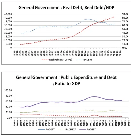
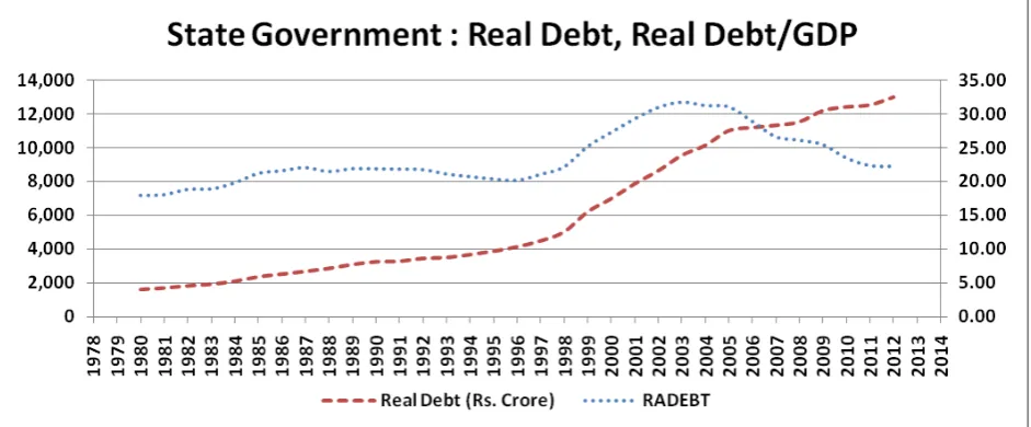
Figures 1, 2 and 3 in the appendix show the time path of components of government expenditure and public debt, as nominal variables (percentage to GDP) and real values respectively for the Centre, General Government and State Governments respectively. In case of the Centre and the General Government, the Debt/GDP ratio is sixty and eighty per cent for the Central and General Government respectively. This is much higher when compared to the Debt/GDP for the State Government; thirty two per cent.
4.2 Methodology
Testing for causality or for cointegration between the two variables is done in three steps. The first step is to verify the order of integration of the variables since the causality tests are valid if the variables have the same order of integration. Standard tests for the presence of a unit root based on the work of Dickey and Fuller (1979) and KPSS (1992) are used to investigate the degree of integration of the variables used in the empirical analysis. The
second step involves testing the cointegration using Johansen’s (1992, 1995) multivariate method to estimate the long-run relation between debt to GDP ratio (bt) and Capital
expenditure (g1). Under this approach, a system of n endogenous variables can be
parameterized into a vector error correction model:
1 1 2 2 .... 1 1
t t t k t k t k t t
X X X X X D u
(22)
where Xt is an (n×1) vector; Гi and П are (n × n) coefficient matrices; Dt are deterministic
components, such as seasonal and impulse dummies; µ is a constant term; k is the lag
20
system, Xt = [ bt , g1] is a (2×1) vector, and Гi and П are (2× 2) coefficient matrices. A cointegrated system implies that П = αβ’ is reduced rank, r, for r < n.
The third step involves utilization of the vector error-correction modelling (VECM) and testing for exogeneity. Engle and Granger (1987) exhibit that in the presence of cointegration, there always exists a corresponding error-correction representation which implies that changes in the dependent variables are a function of the level of disequilibrium in the cointegration relationship, captured by the error-correction term.
As a preliminary analysis to the cointegration tests, we calculate the Karl Pearson’s
coefficient of correlation between g1and bt for the Centre, State and General Government
respectively. Column 2 of Table 2 in A.1.2 shows the results in tabular form. Public debt/GDP and capital expenditure/GDP share an inverse relationship for the Central and General government, while the coefficient in case of the State Government is too low to be interpreted. The vice versa is true for current expenditure to GDP for all the three levels of Government. Thus, in the Indian case, expenditures of productive type could be capital expenditures. However, we confirm this supposition by means of the cointegration and VECM analysis.
4.3 Analysis and Findings
21 4.3.1 Unit Root Tests
The uni-variate time-series properties of capital expenditure/GDP (g1) and public
debt/GDP (bt ) are examined using the unit root tests developed by KPSS (1992) and the
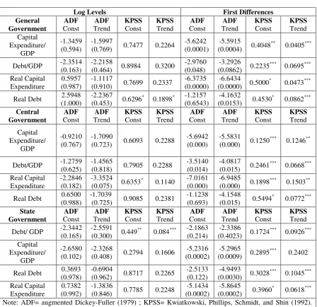
augmented Dickey Fuller (1979). The KPSS tests the null of stationarity, whereas the ADF tests the null of the unit root. If the KPSS test rejects the null but the ADF test does not, both tests support the same conclusions; that is, the series in question is a unit root process. Results of the ADF and KPSS tests are reported in A.1.2 in Table 3 and yield similar results for the Consolidated General Government and Central Government.
In the case of Consolidated General Government and the Central Government, the ADF tests cannot reject the unit root null in any of the indexes (ratio/log level) and the KPSS tests reject the null of stationarity for all indexes. At the first differences, the ADF reject the unit root for g1 and btwhile the KPSS tests support the hypothesis of stationarity. Thus,
ADF and KPSS tests confirm that both debt and capital expenditure are unit root processes and seem to be I(1) at 5 per cent level of significance for the Central and Consolidated General Government. In case of the state level analysis, the first differences seem to be I (2). Hence, the State government data of ratio to GDP variables is excluded in further analysis.
4.3.2 Cointegration Tests
22
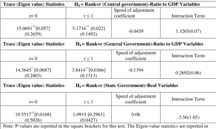
Table 5 in A.1.2 shows the trace and Eigen-value tests for the cointegration rank r, for the two variables. For the consolidated General government and the Central Government, both the tests indicate 1 cointegrating equation at 0.05 levels. This means that bt and g1 are
cointegrated. Apart from the Johansen test we also perform the Engle-Granger test for cointegration since we have only 2 variables. The residuals are stationary for the Centre and the consolidated general government confirming the presence of a cointegration between the two variables. We infer from the fact that capital expenditure/GDP and public debt/GDP are cointegrated, (1) that there is a long-run equilibrium relationship between the two time series and (2) the existence of causality in at least one direction. Furthermore, the deviations of these variables from the equilibrium are stationary, with finite variance, even though the series themselves are non stationary and have finite variance.
In case of the Central Government, the loading factor, which also measures the speed of adjustment back to the long-run equilibrium value is correctly signed (negative). This implies that the long-run equilibrium deviation has a significant impact on public debt. The public debt adjusts at the rate of 0.04 percentage points every year to achieve long-run equilibrium when there is a deviation from the equilibrium. In case of the Consolidated General Government, the loading factor is negative as well and public debt adjusts at the rate of less than 0.13 percentage points every year to achieve long-run equilibrium when there is a deviation from the equilibrium.
4.3.3 VECM Model
We reparametrize the VAR into a vector error correction model using the Johansen framework. Table 6 in A.1.2 shows the results of the VECM representations. The overall R2 is 0.70 and 0.61 respectively for the Consolidated and Central Governments respectively.
The coefficient of the cointegration equation is significant in case of the General and Central Government with low standard errors. The positive sign suggests that changes in capital expenditure adjust in the same direction to the previous period’s deviation from
23
variables. It also means that 0.20 and 0.05 percentage points of disequilibrium in case of general government and Central Government respectively is corrected is corrected within one year.
The coefficient represented in the last column of Table 6 shows that in case of Consolidated general government and the Central Government helps in understanding, the level of adjustment / disequilibrium corrected in the public debt to GDP by a change in the capital expenditure. Thus, a 1 per cent increase in capital expenditure reduces public debt by 0.84 per cent, in the long run for the Consolidated General Government. In case of the Central Government, an increase of 1 per cent in capital expenditure reduces public debt in the long run by 0.09 per cent. This also confirms the inverse relationship between the two variables.
5. Discussion and Policy Implications
Debt sustainability has become a very vibrant issue in the current world scenario with many industrialized countries succumbing to unsustainable budget deficits and debt levels. However, the approach towards implementation of austerity measures is focussed on wage and expenditure cuts. In this paper, the relationship between productive public expenditure and public debt is analyzed using inter-temporal optimization. This is followed by an empirical exercise that using Indian government data analyzes whether specific components of public expenditure do share a long-run relationship with debt and if the relationship in itself is inverse.
The theoretical analysis in the paper shows that when the share of productive expenditure in total public expenditure (phi) is less than 0.5, for the inverse relationship between phi
and debt to hold, stimulus for private investment must also be present in the economy. However, this should only continue till the point when the optimal level of phi is reached.
Beyond the optimal level, an increase in phi might be able to reduce public debt. However,
24
expenditure, where a shift towards an ‘objectively’ more productive type of expenditure, may not raise the growth rate if its initial share is too high. The empirical analysis of the paper shows that capital expenditure of the Indian government shares an inverse long-run relationship with Indian Sovereign debt while the relationship is vice versa for current expenditures. The cumulative analysis of the paper’s findings points towards a possible
complementarity between public and private investment/capital expenditures for reducing public debt in the long run.
25
References
Agénor, P. R., & Neanidis, K. (2006). The allocation of public expenditure and economic growth. Centre for Growth and Business Cycle Research Discussion Paper Series,
University of Manchester, (69).
Ahya, C., Xie, A., Roach, S. S., Sheth, M., and Yam, D. (2006), India and China: New Tigers of Asia, Special Economic Analysis. Morgan Stanley Research.
Alesina, A. F., & Perotti, R. (1999). Budget deficits and budget institutions. In Fiscal
institutions and fiscal performance (pp. 13-36). University of Chicago Press.
Asher, M. G. (2012). Public debt sustainability and fiscal management in India. Public
Debt Sustainability in Developing Asia, 139.
Atkinson, A. B., & Stern, N. H. (1974). Pigou, taxation and public goods. The Review of
economic studies, 119-128.
Atkinson, A. B., Stiglitz, J. E., & Atkinson, A. B. (1980). Lectures on public economics.
Barrios, S., Langedijk, S., & Pench, L. (2010). EU Fiscal Consolidation After the Financial Crisis-Lessons from Past Experiences. Fiscal Policy: Lessons from the Crisis, 561-593.
Barro, R, J., (1990). Government Spending in a Simple Model of Endogenous Growth, Journal of Political Economy, 98(5), pp. S103-26.
Barro, R.J., (1991). Economic growth in a cross section of countries, Quarterly Journal of Economics, 106, pp. 407-443.
Blanchard, O., & Perotti, R. (1999). An empirical characterization of the dynamic effects
of changes in government spending and taxes on output (No. w7269). National bureau of
26
Bose Niloy, Haque E , Denise O.,(2003), Public Expenditure and Economic Growth: A Disaggregated Analysis for Developing Countries. Manchester School75, 5(2007): pp.
533-556
Buiter, Willem H & Patel, U, 1994. Indian Public Finance in the 1990s: Challenges and Prospects, CEPR Discussion Papers 920, C.E.P.R. Discussion Papers.
Carranza, L., Daude, C., & Melguizo, Á. (2014). Public infrastructure investment and fiscal sustainability in Latin America: Incompatible goals?. Journal of Economic
Studies, 41(1), 29-50.
Cavallo, E., & Daude, C. (2011). Public investment in developing countries: A blessing or a curse?. Journal of Comparative Economics, 39(1), 65-81.
Chakraborty, L., Singh, Y., & Jacob, J. F. (2012). Public Expenditure Benefit Incidence on
Health: Selective Evidence from India (No. 12/111).
Chamley, C. (1986). Optimal taxation of capital income in general equilibrium with infinite lives. Econometrica: Journal of the Econometric Society, 607-622.
Chatterjee, S., & Turnovsky, S. J. (2005). Financing Public Investment through Foreign Aid: Consequences for Economic Growth and Welfare*. Review of International
Economics, 13(1), 20-44.
Chatterjee, S., & Turnovsky, S. J. (2007). Foreign aid and economic growth: The role of flexible labor supply. Journal of Development Economics, 84(1), 507-533.
27
Caldara, D., & Kamps, C. (2008). What are the effects of fiscal policy shocks? A VAR-based comparative analysis.
Devarajan S, Swaroop A.M., Zou H(1996) , The Composition of Public Expenditure and Economic Growth, in Journal of Monetary Economics, 37, pp. 313-344.
Dickey, D.A. , Fuller W.A., (1979), Distributions of the estimators for autoregressive time series with a unit root, Journal of the American Statistical Association 74, pp. 427-31.
Engle, R.F. and C.W.J. Granger (1987), Cointegration and Error-Correction: Representation, Estimation, and Testing, Econometrica55 (March), pp. 251-276
Fumio Hayashi & Christopher Sims, (1980), Efficient Estimation of Time Series Models with Predetermined, Discussion Papers 450, Northwestern University, Center for Mathematical Studies in Economics and Management Science.
Goyal, R., Khundrakpam, J.K., Ray P. (2004) ‘Is India's public finance unsustainable? Or,
are the claims exaggerated?’, Journal of Policy Modeling, 26 (3), pp. 401–420.
Giuliodori, M., & Beetsma, R. M. (2004). What are the spill-overs from fiscal shocks in Europe? An empirical analysis.
Gregory, A. and Hansen, B. (1996) , Residual-based tests for cointegration in models with
regime shift’, Journal of Econometrics, 70, 99-126.
Gupta S, Clements B, Baldacci E, Granados C. (2005), Fiscal Policy, Expenditure Composition, and Growth in Low-Income Countries, Journal of International Money and Finance 24, pp. 441-463.
28
Herndon, T., Ash, M., & Pollin, R. (2014). Does high public debt consistently stifle economic growth? A critique of Reinhart and Rogoff. Cambridge journal of
Economics, 38(2), 257-279.
Jha, R., Sharma, A. (2004), ‘Structural Breaks and Unit Roots: A Further Test of the Sustainability of the Indian Fiscal Deficit’, Public Finance Review 32, pp.196-219..
Johansen, S., (1992), Determination of cointegration rank in the presence of a linear trend, Oxford Bulletin of Economics and Statistics 54, pp.383-97.
Johansen, Søren, 1995. A Statistical Analysis of Cointegration for I(2) Variables, Econometric Theory, Cambridge University Press, vol. 11(01), pages 25-59, February.
Kaur, Balbir., & Mukherjee, Atri. (2012). Threshold Level of Debt and Public Debt Sustainability: The Indian Experience. Reserve Bank of India, 1.
Khan, M. S., & Kumar, M. S. (1997). Public and private investment and the growth process in developing countries. Oxford Bulletin of Economics and Statistics, 59(1), 69-88.
Kwiatkowski, D.,Phillips P.,Schmidt P., and Shin Y.,(1992), Testing the null hypothesis of stationarity against the alternative of a unit root, Journal of Econometrics 54, pp.159-78.
Landau, D. (1983), Government Expenditure and Economic Growth : A Cross Country Study, Southern Economic Journal, 49, pp 783-792.
Ortiz, I., & Cummins, M. (2013). The age of austerity: a review of public expenditures and adjustment measures in 181 countries. Available at SSRN 2260771
29
Phillips, P.C.B and P. Perron (1988), Testing for a Unit Root in Time Series Regression, Biometrika, 75, 335–346.
Pitchford, J. D., & Turnovsky, S. J. (Eds.). (1977). Applications of control theory to
economic analysis. Amsterdam: North-Holland.
Pradhan, B. K., Ratha, D. K., & Sarma, A. (1990). Complementarity between public and private investment in India. Journal of Development Economics,33(1), 101-116.
Ramsey, F. P. (1928). A mathematical theory of saving. The economic journal, 543-559.
Reinhart, C. M., & Rogoff, K. S. (2010A). From financial crash to debt crisis (No.
w15795). National Bureau of Economic Research.
Reinhart, C., & Rogoff, K. (2010B). Debt and growth revisited.
Romer, C. D., & Romer, D. H. (2007). The macroeconomic effects of tax changes:
estimates based on a new measure of fiscal shocks (No. w13264). National Bureau of
Economic Research.
Seccareccia, M. (2012). Financialization and the transformation of commercial banking: understanding the recent Canadian experience before and during the international financial crisis. Journal of Post Keynesian Economics, 35(2), 277-300.
Søren Johansen & Katarina Juselius, 1990. Some Structural Hypotheses in a Multivariate Cointegration Analysis of the Purchasing Power Parity and the Uncovered Interest Parity for UK, Discussion Papers 90-05, University of Copenhagen. Department of Economics.
30
Theil, H. (1958). Economic Forecasts and Public Policy. Amsterdam, North.
Tinbergen, J. (1952). On the theory of economic policy.
Topalova, P., & Nyberg, D. (2010). What level of public debt could India target?.
International Monetary Fund.
Turnovsky, S. J. (2000). Methods of macroeconomic dynamics. Mit Press.
Appendix 1
Note on usage of Real Variables
The tables presented in Appendix A.1.2 show the empirical analysis for ratios to GDP of capital expenditures, current expenditures and public debt. Additionally, the analysis with real variables is also presented in the appendix. While no reference is made to real variables in the body of the paper, each of the analysis carried out for the ratio to GDP variables was also done for their real counterparts.
31
[image:32.595.84.553.127.379.2]A.1.1 Figures
Figure 1. Central Government: Major Fiscal Variables (Source: Authors Elaboration on RBI data as mentioned in Table 1)
32
Figure 2. General Government: Major Fiscal Variables (Source: Authors Elaboration on RBI data as mentioned in Table 1)
33
Figure 3. State Government: Major Fiscal Variables (Source: Authors Elaboration on RBI data as mentioned in Table 1)
Notes: RADEBT refers to Debt/GDP, RACUEXP refers to Current exp/GDP and RACAPEXP refers to Capital expenditure/GDP
34
A.1.2 Tables
Table1. Description of Variables
Variables used Type of Government Source
Capital Expenditure Centre, State and General Government RBI Handbook of Statistics on Indian Economy (2013-14)
Current expenditure Centre, State and General Government
RBI Handbook of Statistics on Indian Economy (2013-14) & CSO (National Accounts statistics) Public Debt Centre, State and General Government RBI Handbook of Statistics on Indian Economy (2013-14)
GDP Centre and General Government RBI Handbook of Statistics on Indian Economy (2013-14)
NSDP State Government Indian Public Finance Statistics (2013-14)
GDP Deflator Centre, State and General Government IMF Online Statistics on Indian Economy 2013-14
(Source: Author’s elaboration on data sources mentioned in Table 1)
Table2. Karl Pearson’s correlation coefficient of Current and Capital expenditure with Public Debt
(Source: Authors Elaboration on RBI data as mentioned in Table 1)
General Government Central Government State Government Current
Exp & Debt
Capital Exp & Debt
Current Exp & Debt
Capital Exp & Debt
Current Exp & Debt
Capital Exp & Debt
Ratio
/GDP 0.79 -0.63 0.75 -0.63 0.62 -0.08
Real Variab
les
0.97 0.92 0.98 0.67 0.96 0.94
35
Table 3. Augmented Dickey-Fuller and Kwiatkowski, Phillips, Schmidt, and Shin Tests for Capital Public Expenditure and Public Debt.(Real and Ratio to GDP Variables)
Log Levels First Differences
General Government ADF Const ADF Trend KPSS Const KPSS Trend ADF Const ADF Trend KPSS Const KPSS Trend Capital Expenditure/ GDP -1.3459
(0.594) -1.5997 (0.769) 0.7477 0.2264 -5.6242 (0.0001) (0.0004) -5.5915 0.4048** 0.0405***
Debt/GDP -2.3514 (0.163) -2.2158 (0.464) 0.8984 0.3200 -2.9760 (0.048) (0.0862) -3.2926 0.2235*** 0.0695*** Real Capital
Expenditure (0.987) 0.5957 -1.1117 (0.910) 0.7699 0.2337 -6.3735 (0.0000) (0.0000) -6.6434 0.5000* 0.0473*** Real Debt (1.000) 2.5948 -2.2367 (0.453) 0.6296* 0.1898* -1.2157
(0.6543)
-4.1632
(0.0153) 0.4530* 0.0862***
Central Government ADF Const ADF Trend KPSS Const KPSS Trend ADF Const ADF Trend KPSS Const KPSS Trend Capital Expenditure/ GDP -0.9210 (0.767) -1.7090
(0.723) 0.6093 0.2288
-5.6942 (0.000)
-5.5831
(0.000) 0.1250*** 0.1246**
Debt/GDP -1.2759 (0.625) -1.4565 (0.818) 0.7905 0.2288 -3.5140 (0.014) -4.0817 (0.015) 0.2461*** 0.0668*** Real Capital
Expenditure -2.2846 (0.182) -3.3524 (0.075) 0.6353* 0.1140 -7.0161 (0.000) -6.9485 (0.000) 0.1898*** 0.1503** Real Debt (0.988) 0.6500 -1.7039 (0.725) 0.9085 0.2381 -1.1238 (0.693) -4.1548 (0.015) 0.5494* 0.0772***
State Government ADF Const ADF Trend KPSS Const KPSS Trend ADF Const ADF Trend KPSS Const KPSS Trend Debt/ GDP -2.3442 (0.165) -2.5591 (0.300) 0.449** 0.084*** -2.1863 (0.214) (0.4023) -2.3386 0.1724*** 0.0926***
Capital Expenditure/
GDP
-2.6580
(0.102) -2.3268 (0.408) 0.2794 0.1606 (0.0002) -5.2316 (0.0009) -5.2965 0.2895*** 0.2402
Real Debt (0.978) 0.3693 -0.6904 (0.962) 0.8717 0.2265 -2.5133 (0.122) (0.0030) -4.9493 0.3028*** 0.1045*** Real Capital
Expenditure (0.992) 0.7382 -1.3836 (0.846) 0.7785 0.2248 (0.0002) -5.1434 (0.0002) -5.8645 0.3960* 0.0618*** Note: ADF= augmented Dickey-Fuller (1979) ; KPSS= Kwiatkowski, Phillips, Schmidt, and Shin (1992). The ADF tests are conducted by setting a lag length (k) of 7 as explained in the test. The KPSS tests are reported on the automatic (k) selection of 4 since the sample is small. The ADF tests, ADF Const denotes the only constant term in the estimating equation, whereas Trend denotes both the constant term and linear time trend. For ADF Trend log values of variables have been used. Same notations are used for constant and trend in the KPSS model. P-values are reported in brackets
Critical Values:
ADFConst ADFTrend KPSSConst KPSSTrend
1% -3.73 -4.33 0.739 0.216 5% -2.99 -3.58 0.463 0.146 *** Significant at the 1% level
** Significant at the 5% level * Significant at the 10% level
[image:36.595.82.531.109.543.2]36
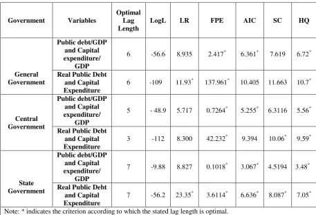
Table 4.VAR Lag Order Selection Criteria (Ratio/GDP and Real variables)
Government Variables
Optimal Lag Length
LogL LR FPE AIC SC HQ
General Government Public debt/GDP and Capital expenditure/ GDP
6 -56.6 8.935 2.417* 6.361* 7.619 6.72*
Real Public Debt and Capital Expenditure
6 -109 11.93* 137.961* 10.405 11.663 10.7*
Central Government Public debt/GDP and Capital expenditure/ GDP
5 - 48.9 5.717 0.7264* 5.255* 6.3116 5.56*
Real Public Debt and Capital Expenditure
3 -112 8.300 42.232* 9.394 10.06* 9.59*
State Government Public debt/GDP and Capital expenditure/ GDP
7 -9.88 8.827 0.1018* 3.067* 4.5194 3.48*
Real Public Debt and Capital Expenditure
7 -56.2 23.35* 3.6114* 6.636* 8.087* 7.05*
Note: * indicates the criterion according to which the stated lag length is optimal. Optimal lag length column indicates lag order selected by the criterion
LR: Sequential modified LR test statistic (each test at 5% level) FPE: Final Prediction error
AIC: Akaike information criterion SC: Schwarz information criterion HQ: Hannan-Quinn information criterion
37
Table 5. Cointegration tests (Selected Variables)
Trace (Eigen value) Statistics H0 = Rank=r (Central government)-Ratio to GDP Variables
r= 0 r ≤ 1 Speed of adjustment coefficient Interaction Term
15.0691**[0.057]
(0.2659) 5.1734
** [0.022]
(0.1492) -0.0459 3.3265(0.07)
Trace (Eigen value) Statistics H0 = Rank=r (General Government)-Ratio to GDP Variables
r= 0 r ≤ 1 Speed of adjustment coefficient Interaction Term
14.5645* [0.0687]
(0.2803) 3.8414
**[0.0366]
(0.1313) -0.1394 0.2692(0.06)
Trace (Eigen value) Statistics H0 = Rank=r (State Government)-Real Variables
r= 0 r ≤ 1 Speed of adjustment coefficient Interaction Term
18.5517**[0.0168]
(0.5026) 1.0915 [0.2961] (0.0427) 0.06 -3.56(1.65)
Note: P-values are reported in the square brackets for this test. The Eigen-value statistics are reported in the round brackets. For the interaction terms, presented in the last column, the value in the round brackets represents the standard error associated with the term. The 5% critical values of the trace statistics for H0 = 0 are 15.49 and for H0 ≤ 1 are 3.84 respectively. The lag lengths used are as per the optimal lag length of Table 3.
*** Significant at the 1% level ** Significant at the 5% level * Significant at the 10% level
(Source: Authors Elaboration on RBI data as mentioned in Table 1)
Table 6. Error Correction Model
General Government R2 Cointegration equation
coefficient Lag 6
D (Capital Expenditure/ GDP) 0.70 0.204***
-0.84** (0.06)
Central Government Cointegration equation coefficient
Lag 5
D(Capital Expenditure
/GDP) 0.61 0.059*** -0.09* (0.237)
State Government Cointegration equation
coefficient Lag 1
D(Real Capital Expenditure) 0.63 -0.005** 0.23** (0.06)
Note: P-values are reported in the square brackets for this test. For the Lag coefficients presented in the last column, the value in the round brackets represents the standard error associated with the term. The 5% critical values of the trace statistics for H0 = 0 are 15.49 and for H0 ≤ 1 are 3.84 respectively. The lag lengths used are as per the optimal lag length of Table 3.
*** Significant at the 1% level ** Significant at the 5% level * Significant at the 10% level
[image:38.595.81.528.495.635.2]38
Appendix 2
A.2.1: VECM (Long Run Properties) and Econometric Relationship between bt and g1
П’s properties explain the long run properties of the VECM model.
Rank (П) =0, non stationary with no cointegration
Rank (П) =2, full rank, which means that the system is stationary as a whole even if individual series are not
Rank (П) =1, non stationary with 1 cointegrating relationships.
For the Johansen test, the rank of the matrix= number of characteristic roots that differ from zero. In case of no cointegration rank of П is 0 and all characteristic roots equal zero. 1-λi= 0.
If rank (П) =1, which is the case in point here, 0 < λ <1, we have the following model
which can be represented as a VAR.
1 2 1
0 1 2
1 2 2
t t t t
t t t t
b b b u
A A A
u
The VECM form hence would be
1 1 1
0 1 2
1 1 2
t t t t
t t t t
b b b u