Study on Distribution Coefficient of Traction Return
Current in High-Speed Railway
Wen Huang, Zhengyou He, Haitao Hu, Qi Wang
School of Electrical Engineering, Southwest Jiaotong University, Chengdu, China Email: [email protected]
Received March, 2013
ABSTRACT
The distribution coefficient of return current network is an important method to decrease the rail potential. In order to resolve the problem of high rail potential in high-speed railway based on EN50122-1 and Pr EN50170 the distribution coefficient of longitudinal traction return current conductors is calculated through changing the interval of transverse connection. Based on field data and theoretical analysis, the parameters of longitudinal traction return current conduc-tors are calculated. Results indicate that the best distance of the transverse connection is 400 m – 600 m.
Keywords: Traction Return Current; Rail Potential; Distribution Coefficient; Interval of Transverse Connection
1. Introduction
Traction return current system consists of the rail, the protective wire (PW) and the integrated grounding line (IGL). It plays an important role in traction power supply system of high-speed railway. The design of the return current network is critical to keep the safe and reliable operation of the traction power supply system. With the popularization of the ballast less track and increase of the traction current, the voltage and the current of the rail are increased accordingly. As one of the traction return channel, the rail is closely related to the safety of the personnel and equipment. High rail potential will cause many problems such as step voltage, touch voltage and the electromagnetic interference with the track circuit [1]. Recently experts had studied on the method which can reduce the rail potential thoroughly [2-6]. Distribution co-efficient of the return current network can reflect the rail potential well. Restrictions on the rail potential are mainly divided into two kinds at present. One is to set up IGL to share the rail potential which is widely used in Germany, France and South Korea. The other uses the rail voltage limiter in Japan who is the earliest developer of high-speed railway [7]. The ideas and concrete tech-nical measures to solve the problem are differed from country to country. A distributed parameter model of rail poten-tial under direct feeding system established with the Matlab/Simulink studied in [8]. It brings in the lo-como-tive coefficient to fix the peak of rail potential. But it does not consider the share of rail current by
longitu-dinal traction return current conductors such as the return line and the IGL in the actual situation. Computational formula of the grounding resistance of the IGL is de-duced in [9]. Furthermore, it studied on the distribution relationship between rail and IGL. However, it didn’t consider the distribution coefficient of the return line in direct feeding system or the PW in the AT system. Cur-rent distribution proportion of the rail, return line and IGL is summarized in [10], in combination with the field test data of the first ballastless track experimental section in China. However, it doesn’t analyze appropriate inter-val of transverse connection systematically.
In China, research on the distribution of longitudinal return current conductors is differed a lot with the actual situation because of without considering environment when the parameters are calculated. Application of the ballastless track in China is just starting out, and there is no experience to design the appropriate transverse con-nection. Therefore, based on the rail, PW and IGL, the parameters of each wire should be calculated respectively in this paper. Combining the field test data in China, re-ferring the related standards in EN50122-1 and prEN- 50170, the optimal design of Chinese high-speed railway traction return system is studied. The most appropriate interval of transverse connection is concluded as well.
2. Traction Return Current System
Traction current is supplied to locomotive through the catenaries by traction substation and returns to traction substation through return current network, forming a complete energy cycle system. In China, high-speed rail- *This work is supported by High-Speed Railway Basic Research Fund
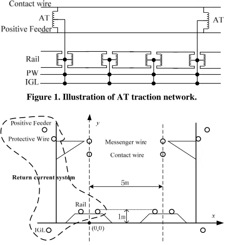
way mainly adopts AT power supply mode, in order to study the distribution of return current system, the interval between each two AT transformers is taken as a study subject as shown in Figure 1.
Traction return current network contains longitudinal traction return current conductors and transverse connec- tions. Among longitudinal traction return current con- ductors, the most important wires are PW, rail, and IGL, the sectional view of traction network as shown in Fig- ure 2.
[image:2.595.58.290.471.722.2]The laying way of PW is overhead and not insulated with pillar, it not only saves the cost in insulating aspect, but also uses the pillar as a good earthling pole. Rail is both running rail and return current conductor. It can be considered that rail is a grounding conductor extending infinitely to both ends. Rail is connected transversely to PW and IGL through the neutral ground terminal of the choke transformer. IGL is an equipotent connecting wire of the integrated grounding system, which is mainly to make the railway electrical and signal devices ground intensively and unify the potential, and usually laid below the ground on both sides of the double-track railway. The environment of each line in return current network is different, and the conductor structure and material have its own characteristic, it must adopt different methods to calculate the parameters for the PW impedance, rail apparent impedance and IGL grounding impedance, respectively. Transverse connections balance the current distribution of return current system, and further to reduce the rail potential, while it meets the design requirements of the integrated grounding system, forming equipotent
[image:2.595.347.499.657.718.2]Figure 1. Illustration of AT traction network.
Figure 2. Sectional view of traction network.
connecting network to facilitate the unification of ground, and traction return channel.
The study on longitudinal return current conductors’ shunt condition still exist a wide gap in actual condition, which is caused largely by the error of the line parameters calculation. Therefore, traction return current network parameters must satisfy the service environment to calculate.
3. Parameters Calculation of Longitudinal
Return Current Conductors
3.1. Impedance of PW
Short distance power line can be used as equivalent circuit model of PW which is made up of steel-cored aluminum strand as one of the longitudinal return current conductors. Equivalent circuit model of PW is shown in Figure 3.
Steel-cored aluminum strand LGJ-120 can be considered to be an example which is very common in high-speed railway in china with equivalent radius and resistance
7.22
e
r mm Km
0.255 /
R . Under power frequency, stranded conductor can be equivalent to solid round wire or tubular round wire by transformation formula. In order to turn the PW into solid round wire, the radius of round which have the same area as the stranded conductor with the current-carrying part are define as equivalent radius [11]. Because of the use of power frequency alternating current in attractive power supply system, the skin effect must be considered. In order to descript the size of the skin effect quantificational, the concept of penetration depth should be considered. Penetration depth can be calculated as
2
503.3
r
f
(1)
where is the angular frequency, is the resistivity of PW, is permeability which Non ferromagnetic materials can be deemed to that 0410 (7 H m/ ).
When return current passed by the PW, skin effect should be taken into account. The internal impedance of the PW can be described as
( 2 ) ( 2 )
2 '( 2 ) '( 2 )
jm ber r jbei r
Z
r ber r jbei r
(2) where and are referred as Kelvin-function, which is one of the Bessel-Function[12]
ber bei
4 8
4 2 8 2
2 6 10
2 6 2 10 2
( ) 1 ...
2 (2!) 2 (4!)
( ) ...
2 2 (3!) 2 (5!)
x x
ber x
x x x
bei x
This expression is too complicated to programmed, so Semlyen and Deri gave a approximate formula to replace, and the error is less than 6%[13], which can be described as
2
PW dc
2
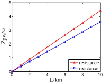
[image:3.595.100.243.88.143.2]Z R Z (3) where the physical significance of Z is the impedance formula that the frequency tend to infinite, it can be de- rived as Z (1 j p) 2 re . The relationship between PW impedance and length is shown as Figure 5.
Figure 4 shows the change law between impedance and length of PW which can be approximate it at the equivalent circuit model of short distance power line. The impact of conductance and susceptance can be ig- nored, so the relationship between PW impedance and length is positive correlation.
3.2. Apparent Impedance of Rail
The monoblock track board of ballastless track which is made up with armored concrete has been widely used in high-speed railway. It leads to a serious defective insula- tion between the rail and earth. Traction current leaks into the earth continually when it pass by the rail, and it forms the rail-earth potential when the current passed by the rail leakage impedance. Rail apparent impedance can not be determined by the series-parallel model of Soil ground resistance and rail impedance. Computing method of rail’s apparent impedance is concluded in 14, which need to analysis the relationship between rail potential and current. Figure 5 shows the model of rail distribu- tion parameters.
The distribution of valid values of the rail current in steady state is described as
0 2 4 6 8 10
0 1 2 3 4 5
resistance reactance
Figure 4. Relationship between protective wire’s impedance and length.
0
( ) 2
rx I e I x
(4)
where I0 is the current which flow into the rail, and r
is attenuation constant of the rail current, which can be described as r (Rr j L r) ( Gr j C r)
According to the rail current distribution function, the rail potential distribution function can be derived as
.
0
( ) ( )
2
rx
r r
r I e
U x R j L
(5)
According to the rule of rail potential distribution, the apparent impedance between two points at rail is deduced as
0
( ) (0) 1
( )
rl
r r gr
r
U l U e
Z R j L j M
I
(6)
where Mgr is the mutual reactance between rail and
[image:3.595.323.520.477.705.2]IGL.
Figure 6 illustrates the relationship between rail ap- parent impedance and length. The rail’s apparent imped- ance becomes bigger and bigger with the increase of the length of the rail, and the reactance value plays a main role. But the impedance tends to steady when the length increase to 2km. The apparent impedance of rail is only 0.2551 j0.8653 when the length of rail increases to 10km, which shows that the rail impedance occupy a little of proportion in traction network.
Figure 5. Equivalent circuit model of rail.
0 2 4 6 8 10
0 0.2 0.4 0.6 0.8 1
resistance reactance
[image:3.595.83.263.566.709.2]3.3. Grounding Impedance of IGL
[image:4.595.340.537.112.219.2]Because of the close relationship between IGL and earth, the impact of soil parameters must be considered when the impedance is calculated.
Figure 7 shows the distributed parameter model of IGL. Based on article 9, mutual reactance is considered in this paper now. It is shown in Figure 7, Rg, Lg, Cg
and Gg are the IGL inherent resistance, inductance,
capacitance and leakage conductance to earth per length, respectively. The current of IGL can be described as
2
0 2
( , ) 2 sin
1
g g g
g
x l x
l
e e e
i x t I t
e
(7)
If we only consider the change of conductor’s current effective value, the current distribution of finite length earthing conductor is derived as
2
0 2
( ) 1
g g g
g
x l x
l
e e e
I x I
e
(8)
where I0 is the current of point M, and the attenuation
coefficient of current is is described as
2 ' ln( ) 2 g l a ha (9)
where ' is the resistivity of IGL, and a is the cross section area of conductor. is the earth resistivity, and
is the burial depth.
h
Because of the close distance of IGL and rail, the mu- tual reactance of IGL and rail must be considered. The potential of IGL is described as
0 0 0 0 ( ) ( ) ( )
(1 ) ( )
(1 ) (1 ) (1 ) g g r r l
M g g g
l r gr l g g l g l gr N N l r
U I x R j L dx
I x j M dx U
e R j L
I e
e j M
I U e
where the mutual reactance can be expressed as
0 2
= (ln 1
[image:4.595.132.228.351.396.2]2 gr gr l l M d ),
Figure 7. Distributed parameter model of IGL.
gr is the distance between IGL and rail. The grounding
resistance is deduced as
d
0
(1 ) ( )
(1 )
ln( )
(1 ) 2
+ (1 ) g g r r M l g g l g l gr l r U Z I
e R j L
e
l
e j M ha
[image:4.595.337.510.568.711.2]l e (10)
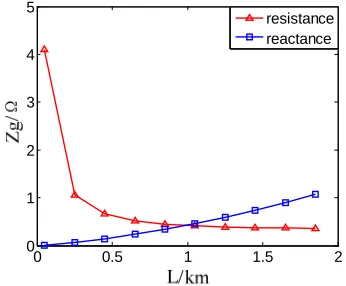
Figure 8 gives the component of grounding resistance decreases rapidly with the increase of the length of IGL. It’s because of the leak conductance between IGL and earth. The component of resistance keeps steady when the length of IGL longer than 1 km. But the component of reactance becomes bigger and bigger with the increase of the length. The size of the grounding impedance de-pends on the value of reactance when the length longer than 1 km.
4. Distribution Coefficient and Interval of
Transverse Connection
In the longitudinal return current conductor, traction cur- rent return to traction substation through three accesses of PW, rail and IGL, the impedance of each conductor determines the proportion of current in each line which is distribution coefficient. Longitudinal return current con- ductors are shown in Figure 9, where ZPW is the im-
pedance of PW, Zr is the impedance of rail and Zg is
the impedance of IGL.
According to the circuit analysis theory, distribution coefficients of each line are shown in Figure 10.
As seen from Figure 11, with length of PW increasing, distribution coefficients of PW are decreasing, which is due to the reason that PW can be seen as a short over- head transmission line that the conductance and suscep- tance are negligible, the resistance value increases as the
0 0.5 1 1.5 2
0 1 2 3 4 5 resistance reactance
Figure 9. Equivalent circuit of traction return current sys-tem.
0 0.5 1 1.5 2
0 0.1 0.2 0.3 0.4 0.5
rail
protective wire
integranted grounding line
Figure 10. Distribution coefficient of traction return current system.
length increases, therefore, the longer the conductor is, the smaller distribution coefficient the PW is. The distri- bution coefficient of rail is increasing within 1 km. On the contrary, the characteristic presents an opposite ten-dency after 1 km, and the value of distribution coefficient reaches the minimum around 1km. The distribution coef- ficient of the IGL increases with the length of the IGL increases and slightly decreases after the distribution coefficient reaches the maximum around 1km.
In the practice, PW, rail and IGL in the longitudinal return current conductor are connected by the transverse connection in a certain interval which leads to realloca- tion of the rail current when it reaches connection point in order to lower rail potential. Rail potential is consid- ered as standards to study the reasonable length between transverse connections. A section of one railway in china is the data source of the rail, ballastless track uses the P60 gapless rail, the impedance of per unit is 4
1.63 10
6.38
r
, the reactance of per unit is ,the leakage conductance of per unit is , depending on the above data, the decay coefficient of rail is
4
5.53 10
5
10 S 2.5
. The average burial depth of IGL is 0.7 m, the av-erage resistivity of soil is
5
10
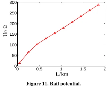
100 m [15]. The other pa-rameters are referring to engineering design standard, traction current is 0 . Figure 11 shows the rail
potential according to the distribution coefficient of rail. 10
I 00 A
It represents the product of distributive current with different rail length and the impedance at this position. According to the EN50122-1 railway applications-fixed equipment-part one and communication system used in the prEN50170, railway regulates that the rail potential is no more than 120 V under the normal operating states
[image:5.595.81.266.187.315.2](t>300 s), and the rail potential is no more than 130 V un- der the normal operating states (t < 300 s)[16]. Fig-ure 11 shows that the rail potential is 129.5 V which rail trans- verse connection interval is 0.65 km, therefore the trans- verse connections interval of rail-PW or rail-IGL should be no more than 0.6 km. The data are shown in Table 1.
Considering the actual situation that rail and IGL are closely contacted with the earth and the current will in- filtrate to the earth by the conductor, the values of distri- bution coefficient of rail and IGL should be smaller than the values in the practice, that is, the value of actual r
should be smaller than that in this table. On the premise of keeping a margin, considering the current-carrying capability and economical efficiency of the PW, rail and IGL, the interval of transverse connection among these three conductors should be designing 400 m - 600 m.
U
5. Conclusions
Based on the PW, rail, and IGL of the longitudinal return current conductors in high-speed railway, the parameters of the wires in different environments were calculated. Combining with the field data and taking relevant require- ments of rail potential in EN50122-1 and prEN50170 as standards, the design which is suitable for traction return current system is concluded, and the optimum transverse connection interval of return current network is obtained.
0 0.5 1 1.5 2
[image:5.595.329.517.428.580.2]0 50 100 150 200 250 300
[image:5.595.306.540.619.725.2]Figure 11. Rail potential.
Table 1. Relationship among the interval of transverse con-nection and shunting coefficient and rail potential.
Transverse interval (m) Distribution
coefficient 350 400 450 500 550 600
PW 0.4265 0.4123 0.3985 0.3852 0.3728 0.3612
Rail 0.4690 0.4605 0.4519 0.4435 0.4356 0.4285
IGL 0.1045 0.1272 0.1496 0.1713 0.1916 0.2103
In consideration of the current carrying capability of each wire, economy and retaining a certain margin, the opti- mum design of transverse interval is between 400 m and 600 m, and the distribution ratio of PW, rail, and IGL is 35%:45%:20%. Rail potential is less than 120 V, which meets the rail potential standards.
REFERENCES
[1] R. Natarajan, A. F. Imece, J. Popoff, K. Agarwalet and P. S. Meliopoulos, “Analysis of Grounding Systems for Electric Traction,” IEEE Transactions Power Delivery, Vol. 16, No. 3, 2001, pp. 389-393.
doi:10.1109/61.924816
[2] A. Mariscotti and P. Pozzobon, “Synthesis of Line Im-pedance Expressions for Railway Traction Systems,” IEEE Transactions on Vehicular Technology, Vol. 52, No. 2, 2003, pp. 420-430.doi:10.1109/TVT.2003.808750
[3] C. F. Yang, J. T. Huang and T. H. Lee, “Effects of Mag-netic Field Induction and Ground Potential Rise on Pilot Wire Relay System Operations,” IEEE Proceedings of Generation, Transmission and Distribution, Vol. 143, No. 3, 1996, pp. 290-294.
[4] R. Cella, G. Giangaspero, A. Mariscotti, et al., “Meas-urement of AT Electric Railway System Currents and Validation of a Multiconductor Transmission Line Model,” IEEE Transactions on Power Delivery, Vol. 21, No. 3, 2006, pp. 1721-1726.
doi:10.1109/TPWRD.2006.874109
[5] S. T. Sobral, G. Azzam and S. C. Sobral, “Ground Poten-tials and Currents in Ubstations Fed Exclusively by Power Cables: An Example Leblon Substation,” IEEE/PES Transmission and Distribution Conference and Exposition, Latin America, Sao Paulo, Brazil, IEEE PES, 2004, pp. 91-95.
[6] S. F. Xie, “Study on Methods to Reducing Rail Potential of High-speed Railway,” Proceedings of 32nd Annual Conference of IEEE Industrial Electronics Society, France, IECON, 2006, pp. 1042-1046.
[7] X. G. Jiang, “Research on Earthing of High Speed
Rail-way,” Southwest Jiaotong University Master Degree Thesis, 2009.
[8] G. Yang, M. G. Liu and N. Li, “Research on Model of Rail Potential Distribution and Its Simulation,” Journal of Beijing Jiaotong University, Vol. 34, No. 2, 2010, pp. 137-141.
[9] G. N. Wu, G. Q. Gao and A. P. Dong, “Study on the Per-formance of Integrated Grounding Line in High-Speed Railway,” IEEE Transactions Power Delivery, Vol. 26, No. 3, 2011, pp. 1803-1810.
doi:10.1109/TPWRD.2011.2117446
[10] Y. Chen and Y. C. Deng, “Analysis of Rail Potential and Current Distribution of Integrated Earthing System for Ballastless Track of Sui-Yu Railway Line,” Journal of Railway Engineering Society, 2007, pp. 426-429.
[11] Q. Z. Li, “Analysis of Tractive Power Supply System,” Southwest Jiaotong University Press, Chengdu, 2007, pp. 243-264.
[12] W. L. Ming and F.Yu, “Numerical Calculations of Inter-nal Impedance of Solid and Tubular Cylindrical Conduc-tors under Large Parameters,” IEEE Proceedings Genera-tion Transmission DistribuGenera-tion, Vol. 151, No. 1, 2004, pp. 67-72.
[13] A. Semlyen and A. Deri, “Time Domain Modeling of Frequency Dependent Three Phase Transmission Line Impedance,” IEEE Transactions, Vol. PAS-104, No. 6, 1985, pp .1549-1555.
[14] G. N. Wu, X. B. Cao and R. F. Li, “Lightning Protection and Grounding of Rail Transit Power Supply System,” Science Press, Beijing, 2011, pp. 230-244.
[15] G. Q. Gao, A. P. Dong and X. Y. Zhang, “Grounding Effect of Integrated Grounding Wire for High-Speed Railway,” Journal of Southwest Jiaotong University, Vol. 46, No. 1, 2011, pp.103-108.