The Kuznets Curve and the Inequality Process

Munich Personal RePEc Archive

The Kuznets Curve and the Inequality

Process

Angle, John and Nielsen, Francois and Scalas, Enrico

The Inequality Process Institute, University of North Carolina at

Chapel Hill, East Piedmont University

12 March 2009

Online at

https://mpra.ub.uni-muenchen.de/16058/

by

John Angle

angle@inequalityprocess.org

Inequality Process Institute

http://www.inequalityprocess.org

Post Office Box 215

Lafayette Hill, Pennsylvania 19444)0215

USA

François Nielsen

Francois_Nielsen@unc.edu

Department of Sociology

University of North Carolina

Chapel Hill, North Carolina 27514

USA

and

Enrico Scalas

Enrico.Scalas@gmail.com

Department of Advanced Sciences and Technology

Laboratory on Complex Systems

East Piedmont University

Via Michel 11, I)15100 Alessandria

Italy

June 29, 2009

Forthcoming in Banasri Basu, Bikas K. Chakrabarti, Satya R. Chakravarty, and Kausik Gangopadhay, eds., ! " # $ " #

)

Four economists, Mauro Gallegati, Steven Keen, Thomas Lux, and Paul Ormerod, published a paper after the 2005 Econophysics Colloquium criticizing conservative particle systems as models of income and wealth distribution. Their critique made science news: coverage in a feature article in &%*". A particle system model of income distribution is a hypothesized universal statistical law of income distribution. Gallegati et al. (2006) claim that the Kuznets Curve, well known to

1. INTRODUCTION

Four economists, Mauro Gallegati, Steven Keen, Thomas Lux, and Paul Ormerod attended the 2005 Econophysics Colloquium and published a paper in its proceedings criticizing conservative particle systems as models of income distribution (Gallegati et al. 2006). Their critique made science news: a feature news article in an issue of &%*". Their paper did a service to research on conservative particle systems as models of income distribution by raising its visibility and

encouraging discussion. We agree with Gallegati et al. that a conservative particle system model of income distribution is a hypothesized universal statistical law. Gallegati et al. assert that the economics literature on the Kuznets Curve shows the unlikelihood that such a law exists. They write that, in economics, relationships between phenomena can change. They claim a conservative particle system cannot account for change. They give the Kuznets Curve as an example of change a conservative particle system cannot explain (Kuznets 1955, 1965). Simon Kuznets won the third Nobel Prize in economics for, inter alia, finding the Kuznets Curve. There is a literature in

economics on the Kuznets Curve which continues today. Neither we nor Gallegati et al. (2006) have seen in this literature a conservative particle system used to explain the Kuznets Curve. See

Nielsen (1994) for a review of Kuznets Curve studies in economics and sociology. Gallegati et al. see explaining the Kuznets Curve as an open problem. Kuznets (1955, 1965) observed that, during the industrialization of an agrarian economy, income inequality first rises and then falls. Gallegati et al. (2006) write that there are “good reasons” for the Kuznets Curve. One reason they cite is the rising proportion of human capital in the labor force. Another is the shift of the labor force out of subsistence agriculture into the modern sector of manufacturing and services. We provide a counter)example to Gallegati et al.’s (2006) claim that a conservative particle system cannot account for the Kuznets Curve. Gallegati et al. have no mathematical model behind the assertion of “good reasons” for the curve. They cite none.

Figure 1 about here

2. THE KUZNETS CURVE

The oldest and best known statistical law of income distribution is the Pareto Law, a broad statement of which is that all size distributions of personal income (in large populations defined geographically) are right skewed with gently tapering right tails, power series tails. In 1954, Simon Kuznets (1955) announced a statistical law of personal earned income, now called the Kuznets Curve. By volume of literature generated, the Kuznets Curve approaches the fame of the Pareto Law.

We examine the Kuznets Curve as the graph of the Gini concentration ratio of personal earned income (or a related income concept such as household income) against the movement of workers from low)skilled, poorly paid work in subsistence agriculture requiring little education into more productive modern sectors of the economy, requiring at least a secondary education and offering higher pay. Social scientists use the word ‘inequality’ casually to name any of several statistics of income when they find the values of these statistics disagreeable. Besides the Gini concentration ratio and the Lorenz Curve of which it is a summary statistic, measures such as %poor, %poor and % rich (with various income cut points for these categories), and dispersion (e.g., variance,

interquartile range) have been used as indicators of inequality. These statistics do not necessarily covary (Wolfson, 1994), who terms the Gini concentration ratio the “gold standard” of income inequality statistics (Wolfson, 1994:353). See Kleiber and Kotz (2003: 20)29, 164) for a discussion of the Gini concentration and the Lorenz Curve.

endpoint. See, for an empirical example, Nielsen (1994: 667), a graph of the Gini concentration of income as a function of the percent of a birth cohort that eventually enrolls in secondary school in 56 countries circa 1970. Figure 1 is a stylized iconic Kuznets Curve.

The present paper shows how a particular conservative particle system model of income distribution gives rise to the iconic Kuznets Curve as the Gini concentration ratio of the mixture of a model agrarian distribution of earned income and a model modern distribution as the mixing

weight goes from 100% agrarian to 100% modern. The particle system generating the model agrarian and model modern earned income distributions is the Inequality Process (Angle, 1983, 1986, 2002, 2006), a conservative particle system. We use Gallegati et al.’s measure of the transition of a labor force from agrarian to modern: the acquisition of human capital as workers move from subsistence agriculture in rural areas to employment in the modern sector in cities. We take into account the greater purchasing power of a unit of currency in rural than in urban areas.

Kuznets (1965) argued that the shift of the labor force from the agrarian sector with low average income to the modern sector with higher average income produces a trajectory of the inequality of income in both labor forces combined that rises, levels off, and declines during the transition. Using point estimates of the agrarian and modern wage, the result follows for the Gini concentration ratio from its definition in the case of discrete observations (Kleiber and Kotz, 2003: 164):

)

1

(

|

|

−

−

≡

∆

∑

∑

n

n

x

x

j i j

n

i

n (1)

where Mn is Gini’s mean difference, xi is the income of the ith recipient in a population of n

recipients. The Gini concentration ratio, Gn:

µ

2

n n

G

≡

∆

where mean income of the population is N. If all agrarian workers earn an income of xa and all

modern workers earn an income of xm, and xm > xa, then the number of nonzero terms contributing

to Mn and Gn, i.e.,| xa–xm | and | xm–xa|, is proportional to pq where p is the proportion of agrarian

workers and q the proportion of modern workers, and p + q = 1. Hence the concave down curve of Gn plotted against q. Since N increases as the proportion, q, of modern workers rises, the concave

down graph of the Gini concentration ratio, G, against q, is skewed to the right.

However, this result is not a satisfactory account of the empirical Kuznets Curve since at the start point and end point of the transition, i.e., p or q equals 0.0 or 1.0, the Gini concentration ratio, (1), equals 0.0, a value of the Gini concentration ratio never seen or approached empirically. At least two more considerations have to be taken into account to generate an empirically relevant Kuznets Curve.

3. Explaining The Empirical Kuznets Curve

3

a) The Kuznets Curve and the Metro)Nonmetro Gap in the Cost of Living in the U.S.

Gallegati et al. (2006) define the transition from agrarian to modern sectors of employment in terms of the education level of the labor force and the migration of labor from rural to urban areas. Nord (2000) estimated the difference in the cost of living between the metro and nonmetro {footnote 1} U.S. in the 1990’s. Joliffe (2006) also estimated this difference. Nord estimated that the cost of living in the nonmetro U.S. was about 84% that of the metro. Joliffe estimated the cost of living in the nonmetro U.S. at 79% that of the metro. Taking the mean of these two estimates at 81.5% implies that $1 of earned income in the nonmetro U.S. has the purchasing power of

approximately $1.23 in the metro U.S. A similar difference in the purchasing power of currency exists between urban and rural areas worldwide. This difference is likely much greater in economies whose labor forces are transitioning out of subsistence agriculture to employment in the modern sector. This transition was made in the U.S. in the 19th and early 20th centuries. The U.S. metro and nonmetro labor forces are similar, although nonmetro wages are lower partly due to a lower cost of living in the nonmetro U.S. and partly due to the somewhat lower level of education of the

nonmetro labor force.

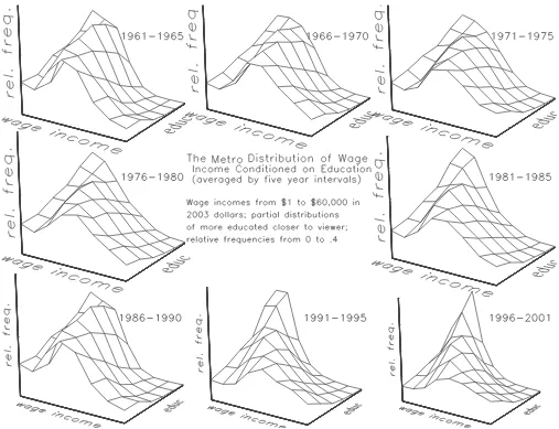
Figures 2 and 3 about here

b) Modern and Agrarian Income Distributions and The Kuznets Curve

The ‘metro’ and ‘nonmetro’ concepts are the nearest approximation to the concepts ‘modern’ and ‘agrarian’ within the U.S. national statistical system. Besides the effect of the cost of living difference between metro and nonmetro areas on wage incomes, there is also the effect of the difference in the distribution of education in the metro and nonmetro labor forces. The distributions of annual wage income conditioned on education in the metro and nonmetro U.S. are similar. See figures 2 and 3. The two parameter gamma pdf offers a good fit to the distribution of annual income in the U.S. conditioned on education in the period 1961)2003 (Angle,1996, 2006). The mixture of the partial distributions of this conditional distribution (each partial distribution weighted by its share of the labor force) has a right tail heavy enough to account for the National Income and Product Account estimates of aggregate wage income in the U.S., an approximately Pareto right tail (Angle 2001,2003). The shape parameters of the gamma pdfs fitted to partial distributions of the distribution of annual wage income conditioned on education scale from low to high with worker education in the whole U.S. (Angle, 1996, 2006; and Table 1).

The two parameter gamma pdf is:

x

e

x

x

f

α

α

λ

Γ

≡

)

(

)

(

where, x > 0, x is interpreted as earned income, α is the shape parameter, λ is the scale

parameter, and (3) is referred to as GAM(α,λ). In terms of a gamma pdf model of earned income distribution of the whole U.S. labor force, a mixture of the metro (m) and nonmetro (nm)

distributions, the Kuznets Curve is the graph of G, the Gini concentration ratio of h(x) plotted

against q, the proportion metro, where h(x) is:

( )

( )

)

,

(

)

,

(

)

(

m m nm nm m m nm nm

GAM

q

GAM

p

e

x

q

e

x

p

x

h

m nm nm nm

λ

α

λ

α

α

λ

α

λ

+

≡













Γ

+













Γ

≡

p + q =1

αnm = shape parameter of the gamma pdf model of the nonmetro wage income distribution

λm = scale parameter of the gamma pdf model of the metro wage income distribution.

The two parameter gamma pdf is not in general closed under mixture, i.e., h(x) is not itself a two parameter gamma pdf unless either p or q = 0.

Table 1. Gamma shape parameters of partial distributions of the distribution of annual wage income conditioned on education in the U.S., 1961)2003. Standard errors of estimate are negligibly small. Source: Angle (2006)

Highest Level of Education Estimate of shape parameter, αi , of ith partial distribution

Eighth Grade or Less 1.2194

Some High School 1.4972

High School Graduate 1.8134

Some College 2.0718

College Graduate 2.8771

Post Graduate Education 3.7329

Most of the workers in the lowest level of education in table 1 were close to the upper limit of that category. A fully agrarian labor force, in the sense of a labor force uninvolved with an industrial economy, would be largely illiterate and, extrapolating from table 1, would have a shape parameter fitted to their earned income distribution distinctly smaller than 1.2 . To extrapolate conservatively, we specify the shape parameter of the gamma pdf of an agrarian distribution of earned income as 1.0. For much of the 20th _{century in the U.S. a high school diploma (completion}

of secondary education) was the standard qualification for industrial, “blue collar” labor. We take the gamma shape parameter of U.S. high school graduates, 1.8, as the model of earned income distribution of the modern sector of an economy.

The Gini Concentration Ratio of a Gamma PDF and a Mixture of Two Gamma PDF’s

McDonald and Jensen (1979) give the Gini concentration ratio, GΓ, of a two parameter

5

(

)

(

1

)

2

1

+

Γ

+

Γ

=

Γ

_π

_α

α

G

GΓ is a monotonically decreasing function of α. GΓ = .5 when α = 1.0. The G of a mixture of gamma

pdfs cannot be expressed, in general, as a linear function of the GΓ’s of the gamma pdf summands.

The GΓ of a gamma pdf is a function of its shape parameter alone. The G of a mixture of two

gamma pdf’s is, in general, a function of all four gamma parameters. There is no simple

expression for the Gini concentration ratio of a mixture of two gamma pdf’s with distinct shape and scale parameters. However, the G of h(x), (4), can be found by numerically integrating the Lorenz Curve of h(x) and subtracting that integral from the integral of the Lorenz Curve of perfect equality. The Gini concentration ratio of h(x) is twice that difference. See Kleiber and Kotz (2003) for a discussion of the Gini concentration ratio as a summary statistic of the Lorenz Curve.

Does the Greater Purchasing Power of Money in the Agrarian Sector Account for the Kuznets Curve? If a unit of currency has greater purchasing power for the agrarian labor force than the modern labor force, an agrarian wage income with purchasing power equal to that in the modern sector is smaller. Assuming that education levels in both the rural and urban labor force were equal, gamma models of the wage income in both sectors will differ only in their scale parameters, i.e., GAM(αM,λM) is the model of the distribution of the modern sector, GAM(αA,λA) the model of the

agrarian sector, αM = αA and λM < λA. Suppose the purchasing power of a unit of currency in the

agrarian sector is twice that of the modern sector, i.e., λA = 2.0 λM . Since the mean of the two

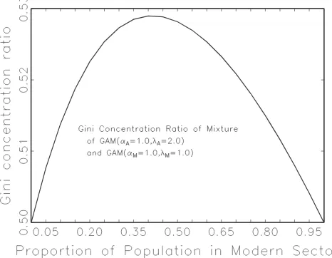
parameter gamma pdf model is α/λ, mean wage income in the modern sector is twice that of the agrarian sector. Figure 4 graphs the Gini concentration ratio of the mixture of the two gamma pdfs, h(x) = p GAM(αA = 1.0, λA = 2.0) + q GAM(αM = 1.0, λM = 1.0), as q, the proportion in the

modern sector, goes from 0.0 to 1.0. Figure 4 shows that when the purchasing power of a unit of currency in the agrarian sector is twice that in the modern sector, that difference alone cannot produce the iconic Kuznets Curve of figure 1. Figure 4 shows 1) the Gini concentration ratios of the 100% agrarian and the 100% modern labor forces as equal, and 2) the Kuznets Curve as nearly symmetric. Thus, figure 4’s hypothesis is not empirically relevant.

Figure 4 about here

Does the Rise of the Educational Level of the Labor Force during the Agrarian )> Modern Transition Account for the Kuznets Curve?

Suppose that there is no difference in the purchasing power of a unit of currency received by a worker in the agrarian sector and a worker in the modern sector (λA = λM = 1.0), but rather there

is a substantial difference in education and a concomitant difference in the shape parameters of the gamma pdfs fitting the distributions of earned income in each sector. Let the shape parameter of the gamma pdf model of wage income distribution in the agrarian sector be αA = 1.0, i.e.,

somewhat smaller than the shape parameter of the gamma pdf fitted to the wage income distribution of U.S. workers with eight years or less of elementary schooling. Let the shape

parameter of the gamma pdf model of wage income distribution in the modern sector be αA = 1.8,

i.e., the estimate of the shape parameter of the gamma pdf fitted to the wage income distribution of U.S. workers who completed high school (secondary education). Figure 5 shows the Gini

concentration ratio of the mixture, h(x) = p GAM(αA = 1.0, λA = 1.0) + q GAM(αM = 1.8, λM = 1.0),

as the mixing weight, q, the proportion in the modern sector, goes from 0.0 to 1.0. Figure 5

demonstrates that a rise in the education level of the labor force in its transition from the agrarian to the modern sectors accounts for the decrease in the Gini concentration ratio of earned income but not for the initial uptick of the curve.

The Joint Effect of Greater Purchasing Power in the Agrarian Sector and A Rise in Education Level in the Agrarian )> Modern Transition Accounts for the Kuznets Curve

The greater purchasing power of a unit of currency accounts for the upward movement of the Kuznets Curve over its left side, i.e., as the fraction of the labor force in the modern sector moves up from 0. The rise in education level of the labor force accounts for the fall in the Kuznets Curve. Suppose the cost of living in the agrarian sector is 81.5% of that of the modern sector. The greater purchasing power of a unit of currency in the agrarian sector would be 1.23 that of the modern sector, using estimates of the greater purchasing power of a U.S. dollar in the nonmetro U.S. than the metro U.S. in the 1990’s. Suppose the education level of the modern sector results in a wage income distribution that is fitted by a gamma pdf with the same shape parameter as that fitted to the wage income distribution of high school graduates (secondary school completion) in the U.S., a gamma shape parameter of 1.8 . The graph of the Gini

concentration ratio of h(x) = p GAM(αA = 1.0, λA = 1.23) + q GAM(αM = 1.8, λM = 1.0) is shown in

figure 6. Figure 6 contains both defining features of the iconic Kuznets Curve, the initial uptick in the Gini concentration ratio over a small proportion of the labor force in the modern sector followed by a long, nearly linear decline to the lower Gini of the modern sector as the proportion of the labor force in the modern sector rises. If the cost of living in the agrarian sector is somewhat lower than 81.5% that of the modern sector – say 2/3, and if there is the difference in education levels of figures 5 and 6, then figure 1 results. Figure 1 is the iconic Kuznets Curve of the introduction to this paper. So, if a conservative particle system can account for a) the approximately gamma distribution of wage income, and b) the shape of this distribution by level of education, we have a counter)example to Gallegati et al.’s proposition that a conservative particle system cannot account for the Kuznets Curve. The difference in cost of living by sector is an adjustment that is easily made.

Figure 6 about here

4. The Inequality Process and The Kuznets Curve

The earliest article we have found that develops a statistical mechanical theory of income distribution is Harro Bernadelli’s 1943 article in Sankhyā, “The Stability of the Income

Distribution“, a paper that recognizes that stable features of this distribution indicate its generation by a statistical law. The Inequality Process is a candidate model of that law similar to the Kinetic Theory of Gases particle system model of statistical mechanics (Angle, 1990). The Inequality Process (Angle, 1983, 1986, 2002, 2006) randomly matches pairs of particles for competition for each other’s “wealth”, a positive quantity that is neither created nor destroyed in the particle encounter. The Inequality Process is thus a conservative particle system model, i.e., in the class of model criticized by Gallegati et al. The transition equations of the Inequality Process are:

(6)

where xit is the wealth of particle i at time step t; ωθj ∈(0,1) is the fraction lost in loss by particle j;

ωψi∈(0,1) is the fraction lost in loss by particle i; and dt is a sequence of dichotomous independent

random variables equal to 1 with probability 1/2 and to 0 with probability 1/2.

The provenance of the Inequality Process is a verbal theory of social science (Angle, 1986, 2006) that identifies competition as the generator of income distributions. In particular, the source of the Inequality Process asserts that more skilled and productive workers are more sheltered in this competition, i.e., a particle with smaller ωψ represents a more productive worker.

Consequently, the Inequality Process must show that particles more sheltered from competition have a distribution of wealth that fits the empirical distribution of earned income of more

7

productive workers. We agree with Gallegati et al. that worker education is a measure of worker productivity. The Inequality Process must account for the distribution of earned income conditioned on education. The test of whether it does so is performed by equating an ωψ equivalence class of

particles with observations on workers who report a given level of education and then by fitting the stationary distribution of particle wealth in the ωψ equivalence class to the income distribution of

workers at that level of education. The Inequality Process passes this test (Angle, 2006). Gallegati et al. are concerned about testing a model of the stock form of wealth against data on its flow form, income. Capitalizing aggregate earned income shows that most of the stock of wealth of an industrial economy is in human capital, largely the educations, of its workers. Earned income is the annuitization of human capital. Earned income is closely correlated with human capital. The

substitution of one variable for another one that is closely correlated is well established in economics. See Friedman (1970 [1953]).

The Inequality Process’ stationary distribution of wealth in the ωψ equivalence class is

approximately a gamma pdf (Angle, 1983, 1986, 2002, 2006) for ωψ’s estimated from earned

income distributions conditioned on education:

(7)

where X > 0 represents wealth (income) in the ωψ equivalence class; the shape parameter is

ψ ψ

ψ

_ω

ω

α

≈

1

−

;

t t t

µ

ω

ω

λ

_~

1

−

≈

,

ω

~

Nt the unconditional mean of x at time t. Nψt is the mean of x in the ωψ equivalence class; Nψt

≈

α

/

λ

=

(

ω

~

µ

)

/

ω

.

The Macro Model of the Inequality Process, (7), (Angle, 2007) represents the agrarian distribution of earned income as a gamma pdf with a larger ωψ (smaller αψ) and larger λψt, than

those of the modern distribution, i.e., able to reproduce figure 1, the iconic Kuznets Curve, as the Gini concentration ratio of the mixture of the two pdf’s, h(x):

h(x) = p GAM(αA, λA) + q GAM(αM , λM ),

where the subscript A indicates the agrarian distribution and the subscript M the modern distribution. Reproduction of the iconic Kuznets Curve requires both a lower cost of living in the agrarian sector and a higher education level of the labor force in the modern sector. {footnote 2}

5. Conclusions

The Inequality Process, a conservative particle system, implies its macro model, a model of its stationary distribution in each equivalence class of its particle parameter. The macro model of the Inequality Process (7) presents a counter)example to Gallegati et al.’s claim that the iconic Kuznets Curve is a dynamic empirical income phenomenon a conservative particle system cannot

2 We have not excluded the possibility that other conservative particle system models of income distribution might do the same. Nor do we assert that we have identified all factors that might give rise to an iconic Kuznets Curve. Indeed we think it likely that the left censoring of the income distribution (exclusion of small incomes from tabulation) in countries with small GDP per capita is also involved.

x

t t

e

x

x

f

ψ λ α ψ α ψ

α

λ

explain. Kuznets (1965) thought the curve named after him resulted from the transition of a labor force from employment in the agrarian sector to employment in the modern sector. The macro model of the Inequality Process explains the Kuznets Curve the same way. Its explanation is more satisfactory because more relevant information is included and more of the features of the iconic Kuznets Curve are reproduced. We thank Gallegati et al. (2006) for stimulating discussion and research into particle system models of economic phenomena, indeed for encouraging the present paper. Their paper succeeded in directing attention to the subject of particle system models of income distributions more effectively than publications on the wide empirical relevance of such models. Economists need not fear this class of model. We expect that this line of research will put many of the verbal tenets and basic insights of the paradigm of economics on a firm scientific footing for the first time. We welcome Gallegati et al. as collaborators in this enterprise.

6. References

Angle, John. 1983. "The surplus theory of social stratification and the size distribution of Personal Wealth."

+,-. * "" / & " "* & & & $ & , Social Statistics Section. Pp. 395)400. Alexandria, VA: American Statistical Association.

_____. 1986. "The surplus theory of social stratification and the size distribution of Personal Wealth." $ 0 * " 65:293)326.

_____. 1990. "A stochastic interacting particle system model of the size distribution of wealth and income."

+,,1 * "" / & " "* & & & $ & , Social Statistics Section. Pp. 279)284. Alexandria, VA: American Statistical Association.

_____. 1996. "How the gamma law of income distribution appears invariant under aggregation". 2 %* $ 3 & " & $ $ / . 21:325)358.

_____. 2001. "Modeling the right tail of the nonmetro distribution of wage and salary income". 411+

* "" / & " "* & & & $ & , Social Statistics Section. [CD)ROM], Alexandria, VA: American Statistical Association.

_____. 2002. "The statistical signature of pervasive competition on wages and salaries". 2 %* $ 3 & " & $ $ / . 26:217)270.

_____. 2003. "Imitating the salamander: a model of the right tail of the wage distribution truncated by topcoding . November, 2003 "*" " & " 0" "* $ &&"" & & & $ 3"& $ / , [

http://www.fcsm.gov/events/papers2003.html ].

_____. 2006 (received 8/05; electronic publication: 12/05; hardcopy publication 7/06). The Inequality Process as a wealth maximizing algorithm . 5 & & & $ 3" & $ &

367:388)414 (DOI information: 10.1016/j.physa.2005.11.017).

_____. 2007. The Macro Model of the Inequality Process and The Surging Relative Frequency of Large Wage Incomes . Pp. 171)196 in A. Chatterjee and B.K. Chakrabarti, (eds.), " 3 *6"&

"&7 *6 (Proceedings of the Econophys)Kolkata III Conference, March 2007 Milan: Springer.

Bernadelli, Harro. 1942)44. “The stability of the income distribution”. Sankhyā 6:351)362.

Friedman, Milton. 1970 [1953]. “The methodology of positive economics”. Pp. 3)43 in Essays in Positive Economics. Chicago: University of Chicago Press.

Gallegati, Mauro, Steven Keen, Thomas Lux, and Paul Ormerod. 2006. “Worrying Trends in Econophysics”. Physica A 370:1)6.

9

Kleiber, Christian and Samuel Kotz. 2003. Statistical Size Distributions in Economics and Actuarial Sciences. New York: Wiley.

Kuznets, Simon. 1955. "Economic Growth and Income Inequality." American Economic Review 45:1)28.

______. 1965. Economic Growth and Structure. New York: Norton.

McDonald, James and B. Jensen. 1979. “An analysis of some properties of alternative measures of income inequality based on the gamma distribution function.” Journal of the American Statistical Association 74: 856)860.

Nielsen, François. 1994. "Income Inequality and Development”. American Sociological Review59:654)677.

Nord, Mark. 2000. “Does it cost less to live in rural areas? Evidence from new data on food security and hunger”. Rural Sociology 65(1): 104)125.

11

13

15