Why the saving rate has been falling in Japan

Why the saving rate has been falling in

Japan

Azuma, Yoshiaki and Nakao, Takeo

January 2009

Online at

https://mpra.ub.uni-muenchen.de/62581/

Why the saving rate has been falling in Japan

Yoshiaki Azuma* and Takeo Nakao

(Faculty of Economics, Doshisha University)

Abstract

The paper estimates Japan’s household saving rate function for the 1958−1998 period. We find that the contribution of the increase in net financial assets to the fall of the sav-ing rate varies directly with the amount of assets. This has overwhelmed other factors and has caused the saving rate to fall since 1976.

Key words: Japan’s Household Saving Rate, Income and Financial Assets, Aging of Population, Cointegration Analysis

JEL classification numbers : E 21, C 22

I. Introduction

Japan’s post-war household saving rate rose until the middle of the 1970s, and then has been

fall-ing. In order to explain these phenomena, we analyze the determinants of Japan’s household saving

rate using National Income Accounts data for the 1958−1998 period. This research was originally

mo-tivated by the prolonged slump of the Japanese economy since 1990s. The high saving ratio that had

been an engine to economic growth has now become the major cause of the prolonged

1

slump. Thus

the downward trend that we have now observed in Japan’s saving rate could work as a remedy for

the slump. The matter in question is whether this downward trend will persist or not. From this view

point it is more important than ever to explain why the saving rate has been falling in Japan.

A theoretical prediction of the Life Cycle hypothesis is that the saving rate falls either as the

household wealth rises or the population ages, or both. Thus theory alone cannot answer specifically

why the saving rate has been falling in Japan. In recent empirical studies the negative impact of an

aging population on the saving rate has attracted attention (e.g., Horioka(1997)). We agree that an

ag-ing population must be one of the factors that contributes to the decline in the savag-ing rate. However

we feel that household saving rate may have already started to fall before the onset of an aging

popu-lation.

To clarify this point we first estimate Japan’s household saving rate function using cointegration

analysis. According to the Life Cycle hypothesis we consider disposable income, net financial assets,

────────────

and the proportion of non-working population, which is highly correlated with an aging

2

population.

Then we use the estimates to calculate the contribution ratios of each explanatory variable to the

change in the saving rate. In calculating the contribution ratios we divide the whole sample into the

1958−1976 period, in which the saving rate had risen, and the 1976−1998 period, in which the saving

rate has been falling.

The main results are summarized as follows.

!An increase in household disposable income has a direct effect, and an increase in household net

financial assets has an inverse effect on the saving rate during the whole 1958−1998 period.

!More importantly, the contribution of net financial assets to the change in the saving rate varies

directly with the amount of assets, that is, the higher the amount of household net financial

as-sets, the higher the contribution to the saving rate.

!The proportion of non-working population has an inverse effect on the saving rate, but the

con-tribution is minor compared with either disposable income or net financial assets.

These empirical findings suggest the following explanation for the hump-shaped pattern of Japan’s

post-war household saving rate : although an increase in household disposable income has had a

positive and significant impact on household saving rate, household net financial assets have become

so large that the saving rate has been falling since 1976.

The remainder of the paper is organized as follows. Section II below explains the data. Section III

summarizes the results of the cointegration analysis. Section IV shows the contribution ratios and

concludes by explaining why the saving rate has been falling in Japan. Appendix uses alternative

measure of assets to check the robustness of our finding summarized in section IV.

II. Data

We use calendar year data for the 1958−1998 period. A household saving rate (SHR) is defined as

SH/YD, where SH and YD are the saving and the disposable income, respectively, of households,

in-cluding private unincorporated non-financial

3

enterprises. As a measure of assets we use the closing

balance-sheet account of households, including private unincorporated non-financial enterprises and

private non-profit institutions serving households. From this account we take net financial assets (FA),

net fixed assets (H) and land (L). FA is defined as financial assets minus liabilities and H consists of

mainly residential buildings. SH, YD, FA, H and L are all real magnitude(1985＝100) converted

us-ing the price deflator for private final consumption expenditure. All the data above are taken from 68

SNA, “Annual Report on National

4

Accounts.” We also use the ratio of working population (LPM),

15. The remaining fraction is positively and highly correlated with population

5

aging.

III. Cointegration analysis

Studies in empirical macroeconomics almost always involve nonstationary variables, which causes,

as revealed by Granger and Newbold(1974), a problem of spurious regressions : conventional linear

regression, ignoring serial correlation, of one random walk on another is virtually certain to suggest a

significant relationship, even if the two are, in fact, independent. To deal with this problem, we use

cointegration analysis that consists of unit root tests, cointegration tests, and the estimation of error

correction model.

As Engle and Granger(1987) showed, cointegration is a particularly appropriate way to deal with

this problem. Suppose that two nonstationary sequences are cointegrated, namely, they are integrated

of the same order and the residual sequence is stationary. In this case, even if the two variables are

nonstationary, the model represents a long-run relationship between these two variables. A short-run

adjustment process from the long-run relationship is also derived by taking the residual from the

model of cointegration and by using it as “error correction” terms in the dynamic first-difference

equation. This model is called an error correction model.

Our interest is to analyze the long-run relationship between the saving rate and its explanatory

vari-ables. As shown in the Granger representation theorem, however, the same assumption that we make

to produce the cointegration implies and is implied by the existence of an error correction

6

model.

Thus we will also show the results of error correction model in Step 3.

Step 1 : Unit root tests

The first step of the cointegration analysis is to examine the time-series properties of the data.

Spe-cifically we conduct several unit root tests to see if all variables have unit roots in their levels and are

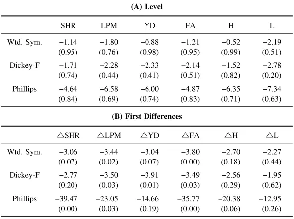
stationary in their first differences. In table 1 we summarize the results (p-values in parentheses) on

the augmented Dickey-Fuller test [Dickey and Fuller(1979)], which is the most widely used, the

aug-mented Weighted Symmetric Tau test [Pantula, Gonzalez-Farias and Fuller(1994)], which is the most

powerful, and the Phillips-Perron test [Phillips and Perron(1988)]. In this table p-values are in

paren-theses and the first differences are expressed by adding △to the top of the variable names. All these

tests include constant term and trend as explanatory variables. Taking first differences of SHR, YD,

FA and LPM produces stationary processes, meaning that all these variables are integrated of order

one, denoted by I(1). At the p-value of p＝0.05, we see that, although H is close to being an I(1)

variable, it fails the test in every case. Therefore we have treated H, as well as L, as a non-I(1)

able.

Step 2 : Cointegration tests and the estimation of the saving rate function

The next step of the cointegration analysis is to test whether these I(1) variables are cointegrated.

For that purpose we obtain an estimate using the cointegration regression suggested by Engle and

Granger(1987). This simply means to estimate household saving rate function using the method of

or-dinary least squares. Given that all variables are I(1), if the error terms are stationary, then the

vari-ables are cointegrated. In this case the estimation result shown in equation (1) is stable in the

long-run and could be interpreted as a model for household saving rate. Notice that, although t-values are

reported in parentheses, we have to be careful in applying t-tests because the residual variance is not

finite.

(1) SHR＝−47.00 (−1.94)

＋0.98 (9.32)

YD− 0.33 (−10.97)

FA＋0.66 (2.33)

LPM,

Adjusted R2

＝0.777, and CRDW＝0.87.

Banerjee, Dolado, Hendry and Smith(1986) [pp. 259−62] showed that, although the estimated

coef-ficients have large biases when the data sample is small, the bias in the coefcoef-ficients as a whole

be-comes small if adjusted R2

is large. In case that the adjusted R2

might be small in this estimation, we

show in appendix an alternative estimation in which we replace net financial assets with the balance

of postal savings and add some other explanatory variables to obtain cointegrated combination of Table 1 Tau-Values in the Unit Root Tests

(A) Level

SHR LPM YD FA H L

Wtd. Sym. −1.14 (0.95) −1.80 (0.76) −0.88 (0.98) −1.21 (0.95) −0.52 (0.99) −2.19 (0.51) Dickey-F −1.71 (0.74) −2.28 (0.44) −2.33 (0.41) −2.14 (0.51) −1.52 (0.82) −2.78 (0.20) Phillips −4.64 (0.84) −6.58 (0.69) −6.00 (0.74) −4.87 (0.83) −6.35 (0.71) −7.34 (0.63)

(B) First Differences

△SHR △LPM △YD △FA △H △L Wtd. Sym. −3.06

variables. In that estimation the adjusted R2

is 0.875 and the main results of the paper still holds.

Hence we assure the small bias in the estimated coefficients.

CRDW is the Cointegration Regression Durbin−Watson statistic introduced by Sargan and

Bhar-gava(1983). The critical value of 1% level for cointegration is about 0.51, and thus the reported

CRDW value of 0.87 indicates the existence of cointegration. We also performed the cointegration

test proposed by Engle and Granger(1987). For the existence of cointegration, p-value should be more

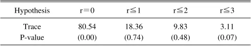
than 0.1, and the actual p-value is 0.63. The most useful cointegration test is the trace test in the

maximum likelihood procedure developed by Johansen(1988) and Johansen and Juselius(1990). Table

2 summarizes the test result in which r denotes the number of cointegrating vectors. This table shows

that the hypothesis that there is one cointegrating vector or less (r≦1) is not rejected, whereas we can

safely reject the hypothesis that there is no cointegrating vector where r＝0. Hence we conclude that

there is a unique cointegrating vector and that equation (1) represents this cointegrating vector.

Step 3 : The estimation of error correction model

Our interest is to analyze the long-run relationship between the saving rate and its explanatory

vari-ables. As shown in the Granger representation theorem, however, the same assumption that we make

to produce the cointegration implies and is implied by the existence of an error correction model,

which is supposed to express the short-run adjustment

7

process. As one of the explanatory variables,

the error correction model has a one-period lagged residual (RES_[t−1]) taken from equation

8

(1). In

deciding the specification of error correction model we use a t-test. Note that, although we cannot use

a standard t-test for RESt−1, Hendry(1986) shows that t-value is still applicable for RESt−1and the

criti-cal value is about 3 in absolute value. In addition, the coefficient of the residual term should be

nega-tive and larger than −1. The estimated result shown in equation (2) satisfies all of these

9

conditions.

(2)∆SHRt＝＋0.43

(2.82)

∆SHRt−1＋0.41

(3.20)

∆SHRt−3＋0.29

(2.08) ∆SHRt−4

＋0.11 (2.25)

∆FAt−2＋1.90

(3.74)

∆LPM− 2.10 (−3.37)

∆LPMt−1＋1.36

(2.66)

∆LPMt−1− 0.54

(−3.90) RESt−1,

R2_＝

0.55, and Adjusted R2_＝

0.45.

Table 2 Johansen’s Maximum Likelihood Trace Test

Hypothesis r＝0 r≦1 r≦2 r≦3 Trace

P-value

80.54 (0.00)

18.36 (0.74)

9.83 (0.48)

3.11 (0.07)

IV. Summary and conclusion : why the saving rate has been falling

We observe that Japan’s household saving rate rose until the middle of the 1970s, and then has

been falling. The estimation result in equation (1) clarifies the factors that affect the saving rate but it

does not by itself explain the rise and fall of the saving rate. Thus we use the estimation result in

equation (1) to calculate the contribution ratios of each explanatory variable to the change in the

sav-ing rate. Table 3 summarizes the results. Note that, in calculatsav-ing the contribution ratios, we divide

the whole sample into the 1958−1976 period, in which the saving rate was rising, and the 1976−1998

period, in which the saving rate was falling (as it has continued to fall to date). Also note that, when

the adjusted R2

is not large enough, the contribution ratios calculated using the fitted values of the

saving rate might not properly explain the actual change in the saving rate. Thus, in parentheses, we

also replace the fitted value of the saving rate with the actual value.

Table 3 suggests the following explanation for the hump-shaped pattern of Japan’s post-war

house-hold saving rate. The rise in househouse-hold disposable income during the 1958−1976 period contributed

greatly to the rise of the saving rate, overwhelming the negative effects of the rise of net financial

as-sets. However, during the 1976−1998 period, the positive effect of the disposable income was still

strong, but was more than offset by the strong negative effect of rising net financial assets. The key

finding here is that the contribution of the increase in net financial assets to the fall of the saving rate

varies directly with the amount of assets, that is, the higher the amount of household net financial

as-sets, the higher the contribution to the fall of the saving rate. Table 3 also clarifies that the

contribu-tion of the aging populacontribu-tion to the fall of the saving rate is minor compared with either disposable

in-come or net financial assets.

Appendix

In this appendix we show an alternative estimation in which adjusted R2

is much higher but a

nar-rower measure of financial assets is used. Specifically we use the balance of the postal savings as a

measure of financial

10

assets. Data on the postal deposit of households are taken from “Monthly Statis-Table 3 Contribution Ratios

YD FA LPM SUM

1958−1976 1976−1998

2.29(1.27) 1.56(1.28)

−0.88(−0.49) −2.24(−1.84)

−0.41(−0.22) −0.31(−0.25)

tics on Postal Services” compiled by Ministry of Posts and Telecommunications.

In this estimation we consider two more explanatory variables : an unemployment rate and a real

interest rate. We consider an unemployment rate as a proxy for liquidity constraints in an aggregate

consumption

11

function. A high unemployment rate decreases the chance of getting new jobs with

higher wages and increases the possibility of being fired. Since both of these effects result in a lower

expected future income, people would increase their saving for future

12

consumption. If this channel is

not negligible, then an increasing unemployment rate after the collapse of the bubble economy has

had an adverse effect on the downward trend of the saving rate. As for a real interest rate, an

in-tertemporal choice of a rational consumer between consumption and saving as well as the Life Cycle

hypothesis implies that the effect of the real interest rate on the saving rate depends on the magnitude

of both income effects and substitution effects.

As for data, unemployment rate (U) is defined as the ratio of totally unemployed persons to the

la-bor force. The data on both the ratio of non-working male persons to total male population with age

larger than 15 and the ratio of totally unemployed persons to the labor force are taken from “Monthly

Report on the Labor Force Survey” by the Statistic Bureau, Management and Coordination Agency.

Real interest rate (R) is defined as nominal interest rate minus inflation rate. The provisional dividend

rate of loan trust (5 years) is used as the nominal interest rate and is taken from “Economic Statistics

Annual.” The inflation rate is measured as the rate of change in the price deflator for private final

consumption expenditure.

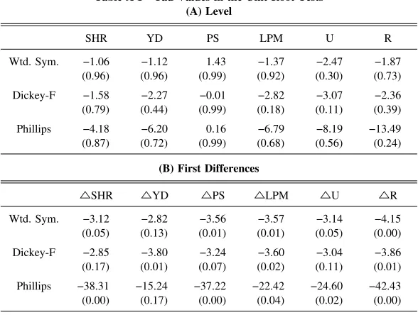
We use calendar year data for the 1957−1997 periods. The results of unit root tests are reported in

Table A 1 Tau-Values in the Unit Root Tests (A) Level

SHR YD PS LPM U R

Wtd. Sym. −1.06 (0.96) −1.12 (0.96) 1.43 (0.99) −1.37 (0.92) −2.47 (0.30) −1.87 (0.73) Dickey-F −1.58 (0.79) −2.27 (0.44) −0.01 (0.99) −2.82 (0.18) −3.07 (0.11) −2.36 (0.39) Phillips −4.18 (0.87) −6.20 (0.72) 0.16 (0.99) −6.79 (0.68) −8.19 (0.56) −13.49 (0.24)

(B) First Differences

△SHR △YD △PS △LPM △U △R Wtd. Sym. −3.12

(0.05) −2.82 (0.13) −3.56 (0.01) −3.57 (0.01) −3.14 (0.05) −4.15 (0.00) Dickey-F −2.85 (0.17) −3.80 (0.01) −3.24 (0.07) −3.60 (0.02) −3.04 (0.11) −3.86 (0.01) Phillips −38.31 (0.00) −15.24 (0.17) −37.22 (0.00) −22.42 (0.04) −24.60 (0.02) −42.43 (0.00)

table A 1, which shows that all variables are I(1).

An alternative estimation to equation (1) is as follows.

(A 1) SHR＝−34.50 (−1.65)

＋0.79 (7.46)

YD − 0.12 (−11.09)

PS＋0.49 (2.01)

LPM＋2.39 (4.26)

U − 0.36 (−4.83)

R,

Adjusted R2_＝

0.875, and CRDW＝1.17.

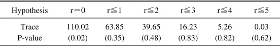
Table A 2 shows the trace test in the maximum likelihood procedure developed by Johansen(1988)

and Johansen and Juselius(1990). In table A 2 we can safely reject the hypothesis that there is no

co-integrating vector, implying that equation (A 1) represents a coco-integrating vector.

Table A 3 shows the contribution ratios of each explanatory variable to the change in the saving

rate. These results are consistent with our main results summarized in section IV.

An estimation of an error correction model is shown in equation (A 2). Since the residual term is

statistically significant, negative, and larger than −1, the equation (A 1) is likely to be a valid

cointe-grating vector.

(A 2)△SHRt＝− 0.26

(−2.42)

△SHRt−3＋0.49

(4.35)

△SHRt−4＋1.40

(3.73)

△YDt−3− 1.55

(−3.36)

△YDt−4

−0.053 (−1.88)

△Wt−4＋1.42

(4.52)

△LPM− 1.54 (−4.79)

△LPMt−1＋1.46

(3.81)

△LPMt−3− 1.50

(−3.91)

△LPMt−4

＋3.09 (3.95)

△U＋1.80 (3.39)

△Ut−3− 1.80

(−3.34)

△Ut−4− 0.26

(−5.96)

△R− 0.26 (−4.63)

△Rt−3− 0.64

(−4.23) RESt−1,

R2

＝0.88, and Adjusted R2

＝0.80.

ACKNOWLEDGMENT

We are grateful to Charles Horioka for valuable comments on earlier drafts. We also benefited from discussions with conference participants in the spring 2004 meetings of the Japanese Economic Association. We also

ac-Table A 2 Johansen’s Maximum Likelihood Trace Test

Hypothesis r＝0 r≦1 r≦2 r≦3 r≦4 r≦5 Trace P-value 110.02 (0.02) 63.85 (0.35) 39.65 (0.48) 16.23 (0.83) 5.26 (0.82) 0.03 (0.62)

Table A 3 Contribution Ratios

knowledge financial support from the “Academic Frontier” Project, 2004−2008, by Japan’s Ministry of Educa-tion, Culture, Sports, Science and Technology (MEXT) and from a special research grant for the promotion of the advancement of education and research in graduate schools provided in 2004 by MEXT and the Promotion and Mutual Aid Corporation for Private Schools of Japan.

Notes

１ Adjusting to a number of conceptual differences and deficiencies in Japan’s National Accounts data, we observe a substantial reduction of Japan’s household saving rate. Even so Japan’s household saving rate is relatively higher than the comparable U.S. saving rate. This result obtains however the aggregate saving rate is defined. See Hayashi(1986, 1997) for detail.

２ In appendix we also consider an unemployment rate and a real interest rate. There are many other factors that might explain the behavior of Japan’s aggregate household saving rate. Cigno and Rosati(1997), for example, finds that, for a given number of people covered, an increase in the average pension level reduces saving in Japan. See Horioka(1992) for a theoretical discussion of a variety of factors that may influence on the downward trend of Japan’s household saving rate.

３ We use household disposable income as an income measure. In lieu of household disposable income, household labor income might be preferable if household total wealth is included as a separate explanatory variable. It is because household disposable income includes capital income accruing to household total wealth. Horioka(1996) uses both measures and obtains qualitatively similar results on household consump-tion funcconsump-tion.

４ The data on Japan’s household saving rate is also available from “household surveys.” The consistency of the data between “National Income Accounts” and “household surveys”, however, is still an ongoing issue. See, for example, Hayashi(1992) for more discussion.

５ Alternatives to the ratio of non-working population such as the sum of the population under the age of 20 and over the age of 60, which we call the number of population not in labor force, or such as the popula-tion over the age of 60, which we call an aging populapopula-tion, are not I(1) variables. Using the data from 1960 to 1997, however, we show that the correlation between LPM and the number of population not in labor force is −0.94. The correlation between LPM and an aging population is −0.90. Besides, if the data on female workers are included in LPM, the correlations fall to −0.73 and −0.65 respectively. In Japan there is a substantial fraction of female workers who work as part-timers and thus we conjecture that the labor force participation rate of female workers has not been stable.

６ For the detail of the Granger representation theorem see Engle and Granger(1987).

７ As shown by Salmon(1982) and Nickell(1985), the error correction model can be derived from the inter-temporal optimization behavior of consumers if we assume the existence of adjustment costs and/or imper-fect information.

８ If the long-run relationship in equation (1) represents a valid cointegrating vector, then RESt−1shows what

proportion of the disequilibrium in household saving rate is corrected in the next period.

９ The general form of the error correction model, when four lags of each explanatory variable are taken from equation(1), is

△SHRt＝Σi＝1βi△SHRt−i＋Σi＝0α1i△YDt−i＋Σi＝0α2i△FAt−i＋Σi＝0α3i△LPMt−i＋γRESt−i.

１０ From 1964 to 1998, the data for personally held total financial assets including postal savings are available from the stock data in Flow of Funds Accounts Based on 68 SNA compiled by the Bank of Japan. Using these data we show that the correlation between postal savings and total financial assets including postal savings is 0.99. This result implies that, during this period, postal savings are good proxy for total financial assets held by household.

１１ See Flavin(1985) and Craigwell and Rock(1995) for the related empirical analyses.

１２ A higher unemployment rate not only lowers the expected future income but also raises the variance of the future income. Hence a higher unemployment rate may increase the saving rate by precautionary saving motive.

Reference

Banerjee, A., Dolado, J. J., Hendry, D. E., Smith, G. W., 1986. Exploring Equilibrium Relationships in Econo-metrics through Static Models : Some Monte Carlo Evidence. Oxford Bulletin of Economics and Statistics 48, 253−77

Cigno, A., Rosati, F. C., 1997. Rise and fall of the Japanese saving rate : The role of social security and intra-family transfers. Japan and the World Economy 9, 81−92

Craigwell, R. C., Rock, L. L., 1995. An aggregate consumption function for Canada : a cointegration approach. Applied Economics 27, 239−249

Dickey, D. A., Fuller, W. A., 1979. Distribution of the Estimators for Autoregressive Time Series With a Unit Root. Journal of the American Statistical Association 74, 427−431

Engle, R. F., Granger, C. W. J., 1987. Co-Integration and Error Correction : Representation, Estimation, and Testing. Econometrica 55, 251−276

Flavin, M., 1985. Excess Sensitivity of Consumption to Current Income : Liquidity Constraints or Myopia? The Canadian Journal of Economics / Revue canadienne d’Economique 18, 117−136

Granger, C. W. J., Newbold, P., 1974. Spurious regressions in econometrics. Journal of Econometrics 2, 111− 120

Hayashi, F., 1986. Why Is Japan’s Saving Rate So Apparently High? NBER Macroeconomics Annual 1, 147− 210

Hayashi, F., 1992. Explaining Japan’s Saving : A Review of Recent Literature. Monetary and Economic Studies (Bank of Japan) 10, 63−78

Hayashi, F., 1997. Understanding Saving : Evidence from the U. S. and Japan. MIT Press.

Hendry, D. F., 1986. Econometric Modelling with Cointegrated Variables : An Overview. Oxford Bulletin of Economics and Statistics 48, 201−12

Horioka, C. Y., 1992. Future trends in Japan’s saving rate and the implications thereof for Japan’s external im-balance. Japan and the World Economy 3, 307−330

Horioka, C. Y., 1996. Capital Gains in Japan : Their Magnitude and Impact on Consumption. The Economic Journal 106, 560−577

Horioka, C. Y., 1997. A Cointegration Analysis of the Impact of the Age Structure of the Population on the Household Saving Rate in Japan. The Review of Economics and Statistics 79, 511−516

Johansen, S., 1988. Statistical analysis of cointegration vectors. Journal of Economic Dynamics and Control 12, 231−254

Johansen, S., Juselius, K., 1990. Maximum Likelihood Estimation and Inference on Cointegration−−With Appli-cations to the Demand for Money. Oxford Bulletin of Economics and Statistics 52, 169−210

Nickell, S., 1985. Error Correction, Partial Adjustment and All That : An Expository Note. Oxford Bulletin of Economics and Statistics 47, 119−29

Pantula, S. G., Gonzalez-Farias, G., Fuller, W. A., 1994. A Comparison of Unit-Root Test Criteria. Journal of Business & Economic Statistics 12, 449−459

Phillips, P. C. B., Perron, P., 1988. Testing for a unit root in time series regression. Biometrika 75, 335−346 Salmon, M., 1982. Error Correction Mechanisms. The Economic Journal 92, 615−629