Inequality factor decompotition under uniform additions property with applications to Cameroonian rural data

(1)

Munich Personal RePEc Archive

Inequality factor decompotition under

uniform additions property with

applications to Cameroonian rural data

Chameni Nembua, Célestin

University of Yaoundé II, Cameroon

2009

Online at

https://mpra.ub.uni-muenchen.de/31250/

(2)

1

INEQUALITY FACTOR DECOMPOSITION UNDER UNIFORM ADDITIONS PROPERTY WITH APPLICATIONS TO CAMEROONIAN RURAL DATA

By

C. CHAMENI NEMBUA

BP 604 Yaoundé, Cameroon [email protected]

Tel (237) 795 19 27

University of Yaoundé II Faculty of Economics and Management Department of Quantitative Techniques

Abstract:

This paper proposes new factors decomposition methods for classical inequality indices such

as Gini index, variance and squared coefficient of variations index. The approach consists in

relaxing the normalization property in order to extend the natural decomposition to a

decomposition rule which satisfies the uniform additions property. The regression-based

method using the new formulations of components contributions is carried out. Empirical

examples, using Cameroonian data, are provided to demonstrate the use of the procedure and

to contrast our results to those based on Morduch and Sicular (2002) principle, especially in

the case of the Gini index.

Keywords: Inequality factors decomposition, uniform additions property, regression-based decomposition, Cameroon.

(3)

2 1- Introduction

Recently, the social dimension as concerns development issues now has a central position in

economic research. Thus, questions on inequality are in awareness. Problems on how to

measure and explain inequality ( among others, Morduch and Sicular 2002, Shorrocks 1980,

Lerman and Yitzhaki 1985) as well as its effects on poverty and economic growth (among

others, Galor and Zeira, 1993; Bourguignon 2004, Shorrocks and Van Der Hoeven 2004) are

gradually ushering themselves on top of the agenda of most researchers in development

Economics.

This rekindled interest on inequality issues re-put on the table the debate on how to analyse

income inequality and its determinants. One of the option retained by researchers was to

aggregate income inequality into an index, such as the Gini index, the variance, the squared

coefficient of variation or the Theil-T index, then undertake a decomposition of this index by

income sources such as salary, transfers, return on investment, etc. Firstly, these researchers

proposed a relatively simple decomposition by income sources that turns out to be a

functional representation linked the structure of the inequality index we are considering (Rao

1969, Fei et al. 1978, Pyatt et al.1980, Fields 1979). In 1982, Shorrocks, in a more general

framework, proposed decomposition by income source that is independent of the considered

inequality index. The Shorrocks method is based on a set of axioms. Shorrocks shows that,

using six axiomatic properties, there exists a single procedure to evaluate the contributions of

the various components of income to total inequality. This result is obtained in two phases.

First, the author shows that there exist an infinite number of decomposition rules applicable to

each inequality index. Second, Shorrocks introduces two particular axioms to obtain the

uniqueness of the decomposition rule. The first of these two axioms is: Normalization for

equal factors distribution which stipulates that: the contribution of all income sources having

an equal distribution is zero. The second axiom states that, if total income is divided into two

components of which one is a permutation of the other, then these two components must have

the same inequality contribution to total income. This axiom is called the two factors

symmetry assumption. Naturally, these two properties have caused a lot of debate.

In this paper, we focus our attention on the first axiom whose implications have been a subject

of controversy between various authors who can be split into two groups. The first group,

(4)

3

axiom is undesirable, especially if the considered measure index is relative. They propose

that, this axiom be replaced by the uniform additions principle ( this principle states that the

contribution of all positive income sources equally distributed be negative) This property

pushes advocates of this group to simply reject all natural decomposition of indices that do

not verify this principle. They propose that the Theil-T index be preferred to the Gini index

just because the natural decomposition of the Theil index verifies the property of uniform

addition while the Gini index does not (for details see Guang Hua Wang 2002).

In opposition to the first group, the second group of authors headed by F.A. Cowell and C.V.

Fiolio (2006) observe that, there is no merit in analysing a decomposition procedure which

satisfies the property of uniform additions. These authors justify the property of normalization

in two ways. Firstly, they remark that it is more sensible that an equally distributed source of

income contribute nothing in accounting for inequality. Secondly, they justify the pertinence

of the property of normalization by the fact, this property enabled Shorrocks to obtain the

unique decomposition of income sources which is independent of the considered inequality

index.

The main objective of this paper is to show how the natural decomposition of some classical

inequality indices can be modified to take into account the property of uniform additions. The

goal here is not to side with either or the other group of authors as concerns the property of

normalization. Our aim is to show that, by relaxing Shorrocks normalization axiom for a

category of inequality indices, we obtain a family of decomposition which verify the property

of uniform additions. In this analysis, we are particularly interested in inequality indices

commonly used in most empirical analysis, such as, the Gini index, the squared coefficient of

variation and the generally entropy family indices. Concerning the first two indices, we

propose a parametric decomposition family with the parameter which is a real function of the

total income. This parameter may be interpreted as the weight of the impact of the uniform

additions on the decomposition approach. When the parameter equal zero, the procedure

yields a decomposition rule (the natural decomposition) which satisfies the Normalization for

equal factors distribution property. In other hand, a value of the parameter greater than zero

leads to a decomposition rule satisfying the uniform addition property; with the sensitivity of

the property in proportion to the magnitude of the parameter value chosen. Hence, our

approach can be seen as the bridge between the proponents and opponents of the property of

uniform additions. In the case of the squared coefficient of variation, the obtained

decomposition family contains the decomposition rule proposed by Morduch and Sicular

(5)

4

Next, we carry the regression-based inequality decomposition method comparable to the

Morduch and Sicular (2002) work. Naturally, this leads to new formula of estimated

contributions of the regression components. We demonstrate our method with data for rural

households in the Centre province of Cameroon which were collected in 2001 by the National

Institute of Statistic.

The outline of the rest of the paper is as follows. Section 2 proposes definitions and main

results. Section 3 is devoted to the regression-based decomposition. As to Section 4, the

preceding results are applied to analyse the rural Cameroonian households’ consumption

inequality. The application is presented in two phases. First, the total households consumption

is broken down into different consumption sources. We compute the contributions to total

consumption inequality of these consumption sources. There, it is found that, the gap is not

sensitive between decompositions rules satisfying the uniform additions property and those

satisfying normalization property. Secondly, we introduce the regression-based with the

constant term to decompose the total income into different determinants. We evaluate the

contribution to the total income inequality of the different determinants, and the results are in

contrast with the first case; the effect of the uniform additions property becomes more

sensitive. Finally we conclude our study in Section 5.

2- Definitions and main results

The starting point is concerned with the inequality measure. We assume that the inequality is

measured by a function I(X)which is continuous and symmetric. The main property can be stated as:

Definition 1: An inequality index I(X) satisfies the property of uniform additions, if for any constant c > o, I(X ce)I(X). Where e



1,1,...,1



is the vector of ones.

The property of uniform additions says that, measure inequality should decrease if everyone

in the population receives an equal transfer. This property has a direct analogism with respect

to the factor decomposition. Suppose now that, there are K different income sources

K

X X

X1, 2,..., so that





 K k

k X X

1

and for any individuali(i1,2,...,n)





 K k

k i

i X

X

1

(6)

5 denote k

S ( k

s ) the absolute (proportional) contribution to the inequalityI(X) of the total income and attributed to the income source k

X .

Definition 2: A decomposition method for a given inequality index I(X)satisfies the property of uniform additions if sk< 0 (sk>0) whenXk ce, where e



1,1,...,1



is the vector of ones and c is a constant greater (less) than zero.

Roughly speaking, inequality decomposition fulfils the property of uniform additions if it

gives strictly negative (positive) contribution to the whole inequality for any income source

that is equally distributed and positive (negative). It is important to note that, satisfaction of

uniform additions property for an inequality index does not necessary imply that any

associated decomposition also satisfies the property as formulate in definition 2. This is

particular the case for the most popular inequality indices such as Gini coefficient, the

coefficient of variation squared and the General entropy family of indices.

We will focus on these inequality indices by examining if their classical decomposition fulfils

the uniform additions property. An alternative decomposition method is proposed when this

property is not satisfied. We will also restrict our attention to the most direct and commonly

used decomposition rules for each index, usually considered as ‘natural decomposition’.

These rules impose (Shorrocks, 1982) on the inequality index to be written as weighted sum

of total incomes:





 n i

i i X x a X

I

1

) ( )

( (1)

Note that the inequality indices mentioned above all satisfy this property.

The absolute contribution of the income source k to the total inequality I(X) is simply:





 n

i

k i i k

x X a S

1

)

( (2)

It is often useful to consider the proportion of the total inequality contributed by different

components. In this case, the proportional contribution of income source k to the overall inequality is :

) (

1

X I

x X a s

n

i

k i i k 





(7)

6

Of course, the method yields an exact decomposition; this means that, the sum of



k K



Sk 1,2,..., equal toI(X) and the sum of the K proportional contributions equal to one.

Considering first the variance (I_VAR) and the coefficient of variation squared (I_CV),

their natural decomposition rules are respectively:











 n

i

i i

VAR x x

n X I

1

1 )

(  for the variance (4) and











 n

i

i i

CV x x

n X I

1 2

1 )

( 

 for the square of coefficient of variation. (5)

The proportional contributions associated to the two indices are identical since the 2_term

cancel in the case of the coefficient of variation:

 k 

CV k

VAR s

s











 

 

n

i

i i n

i

r i i

x x

1 1

 

=





) (

1

X nVar

x x n

i

r i i







=

) (

) , (

X Var

X X

Cov k

(6)

This implies that the proportional contribution of any income source k k(1,1,...,1)

X  which

is equal distributed is

s_VARk s_CVk 

) (

) , (

X Var

X X

Cov k

=

) (

) , (

X Var

e X

Cov k

= 0. (7)

This clearly shows that, the natural decompositions of the variance and the coefficient of

variation squared violate the uniform additions property.

For an alternative decomposition which satisfies the property, we need to rewrite the

expressions (3) or (4) of I_VAR(X)or I_CV(X) as follow:











 n

i

i i

VAR x x

n X I

1

1 )

(  =







 

 

 

 

n

i

i i

i x

x X x

n ₁

) ( 1

1 _ 

(8)

and











 n

i

i i

CV x x

n X I

1 2

1 )

( 

 =











 

 

 

n

i

i i

i x

x X x

n 1

2

) ( 1

1 _ 

 (9)

(8)

7

In the same spirit as above, the corresponding proportional contributions of the income

source k to the overall inequality are now expressed as:





) ( ) ( 1 1 1 X Var x x X x n n i k i i i



         = ) ( ) ( , X Var X X X X X Cov k k        (10)

This alternative decomposition satisfies the property of uniform additions: Suppose that

o

x_i  and that x_ik k o for all i, then,

  k CV k VAR s s







         = ) ( ) ( 1 X Var x x n X n i k i i



       _  = ) ( 1 ) ( 1 X nVar x n X n i i k       



    = ) ( 1 1 1 ) ( 1 X Var x n X n i i k       



    < 0.

An interesting observation that can be made here is that the alternative proportional

contribution rule given in Eq.10 can be related to the former Shorrocks natural decomposition

given in Eq 6 as:

  k CV k VAR s s ) ( ) ( , X Var X X X X X Cov k k        = ) ( ) , ( X Var X X Cov k + ) ( ) ( , X Var X X X X Cov k       _ (11)

This noticeably shows that, the alternative decomposition method corresponds to the natural

decomposition rule and a corrective term. This term, which for the factorXkequal

to _      X X X X Cov k ) (

, , takes into account the link between the total income X and the share

of the factor Xk.

Thus, if _

     X X X X Cov k ) (

, > 0, the contribution of the source k obtained by the alternative

decomposition is greater than its contribution in the natural decomposition rule and inversely.

(9)

8 If the income source k

X is such that X Xk

is not correlated with the total income X (it is

particularly the case where Xk is proportional toX or if Xkis very light relatively to X so

that X Xk

is close to zero), the two methods will practically attribute the same amount of

contribution to the income sources k

X . In contrary, if k

X is evenly distributed (of course it is the case where Xkis constant) with a large total income share, the effect of the second term will be perceptive, and the gap between the two decompositions rules may be sensitive in

proportion to the magnitude of (X).

For (X)1, the proportional contribution rule becomes:





) ( 1 1 1 1 X Var x x x n n i k i i i



        = ) ( , X Var X X X X Cov k k        (12)

On the other hand, if  





 n i i x n X 1 1 )

( , the proportional contribution rule becomes:

  k CV k VAR s s





) ( 1 1 1 X Var x x x n n i k i i i



         = ) ( 1 1 2 2 X Var x x x n n i k i i i



       = ) ( , X Var X X X X Cov k k        (13)

Note that, in this case, the proportional contribution rule coincides with the one proposed by

Morduch and Sicular (2002).

Consider now the Gini coefficient (I_G). If the total income is ordered and individuals

are indexed by their total income rank so that x₁x₂ ,...,x_n, the Gini index can be written:

I_G(X)=



       _  n i i x n i n 1 2 2 1 2  = ( , ) 2 X Rank Cov

n (14) The natural decomposition of the Gini coefficient is then expressed as:



       _   n i k i k G x n i n S 1 2 2 1 2

 (15)

And the corresponding proportional contribution rule is simply:

(10)

9

The corresponding proportional contribution of the source k to the overall inequality is now expressed as: ) ( ) ( 1 2 1 2 1 2 X I x x X n i n s G n i k i i k G



                  = ) , ( ) ( , X Rank Cov X X X X Rank Cov k k        (19) =





) , ( , X Rank Cov X Rank Cov k + ) , ( ) ( , X Rank Cov X X X Rank Cov k        (19b)

The second term in Eq.19b gauges the link between the ranks in the total income and the

share of the income source k X .

This new decomposition satisfies the property of uniform additions. To see it, suppose that

o

xi  and that x o k k

i   for all i, then,

if i₀is the unique integer number such that

2 1

0

  n

i and

(11)

  n i i i X x x a X I 1 ) ( )

( with



  n i i X x a 1 0 )

( and where aX :RR is a strictly increasing

function. And the following proposition states that, the alternative approach leads to a case

where income source decomposition satisfies the uniform additions property.

Proposition 1:

Assume that, the inequality index is a continuous and symmetric functionI(X)which can be

put in the form:





 n i

i i X x x a X I 1 ) ( )

( for any income sourceX ,

with



  n i i X x a 1 0 )

( and where aX :RR is a strictly increasing function. Then,



        n i k i i i X k x x X x a S 1 ) ( 1 )

(  yields an exact factors decomposition which satisfies the

uniform additions property.

Proof: By hypothesis,





 n i

i i X x x a X I 1 ) ( ) ( ,



  n i i X x a 1 0 )

 n i i i X k x x a X 1 1 ) ( ) (  

Since I(X) is symmetric, we suppose that individuals are numbered so that

n

x x

(12)

11



  n i i X x a 1 0 )

( , implies there exists at least one isuch that a_X(x_i)0.

On other side, a_X(x) is different from the null function, and there exist at least one isuch thata_X(x_i)0.

 k i n i i i k x x x n S 1 2 1 1 1    

  0,1 (21)

(13)

12

    

 

    

 

    

 

    

 

      









n

i i

i k

k

x x

n S

1 2

1 1



 

 

=

    

  

      













n

i

n

i i i

k

x n x

n 1 1

1 2

1 1

1 

   



<

_

_

    

  

      









n

i i k

x

n ₁

1

2 1

1 

 

 



< 0 if 1 2

Thus, for1 2, the natural decomposition principle satisfies the uniform additions property. For the limit case 1, which corresponds to the Theil-T index, the uniform additions property is directly satisfied by the natural decomposition since the logarithm

function is concave. Note that, for  2, 2I_(X) is the coefficient of variation squared and we fall again on the decomposition rule given in Eq.13.

All the alternative methods proposed are exact decompositions. They are linked to the natural

decomposition of their corresponding index. However, they reinforce the fact that the

decomposition of an aggregate index may lead to different solutions of the contribution of the

various components. The presence of the parameter(X)corroborates with this situation. Thus, different decompositions of the same index will generate different results during

empirical analyses. The question now posed is : which decomposition method is preferable

and why?

In order to motivate the use of these alternative decompositions, it seems important to study

their properties. Here, we focus our attention on the axiomatic properties of the natural

decomposition defined by Shorrocks (1982).

1.2- Axiomatic properties

If K disjoint and exhaustive income sources are considered, the contribution of the

income source k to the total inequality can be written Sk



X1,X2,...,XK;X;K



and the

proportional contribution is sk



X1,X2,...,XK;X;K



.

The standard axioms for such a contribution function are:

(14)

13

CONT insures that minor observational errors in incomes sources will generate minor

changes in the contribution level.

Axiom2: (Symmetric treatment of income sources, SYM)



X X X X K



TFS recommends that any income source and its permutation must be treated symmetrically

and then assigned the same contributions value. This property was initiated by Shorrocks

(1982) as an assumption on the income factor contribution function. Shorrocks used this

(15)

14 Axiom 6: (Exact decomposition, ED)



1, 2,..., ; ;



( )

1 X I K X X X X

Sk K

K

k







or



1, 2,..., ; ;



1

1 



 K X X X X

sk K

K

k

Proposition 2:

1) The alternative income source decomposition of the Variance and the Coefficient of Variations squared given in Eq.10 satisfies CONT, SYM, ILD, PSYM, TFS and ED.

2) The alternative income source decomposition of the Gini coefficient given in Eq.19 satisfies CONT, SYM, ILD, PSYM, ED but not TFS.

3) The natural decomposition of the General Entropy family of indices given in Eq.22 and the natural decomposition of Theil-T index satisfy CONT, SYM, ILD, PSYM, ED but not TFS.

Proof: Since the proof is similar for the three cases, we will adopt only the case of I_VAR and

CV

I .



X X X X K



s_VARk 1, 2,..., K; ; =

s_CVk



X1,X2,...,XK;X;K



=s_Vark s_CVk 







         ,

Hence it is straightforward that CONT, SYM, ILD, PSYM and ED are satisfied. For TFS, we have seen that:



X X X X K



s_VARk 1, 2,..., K; ; = s_CVk



X1,X2,...,XK;X;K



=

) ( ) ( , X Var X X X X X Cov k k       

,

1 1

M X X Var

X M X

M X M X X M

X X M X Cov



   

 

 



 

= s_VAR1



X1M,X1;X1X1M;2



■

Another desirable property of income source decomposition is the additions stability of

contributions. This property can be defined as follow:

Definition3: If axiom 3 holds, that is the contribution Sk



X1,X2,...,XK;X;K



=S(Xk,X) of the income source k is independent of the degree of disagreggation of the total incomeX , The decomposition method satisfies the additions stability property if ,

for any couple 1 2

,X

X of income sources, S(X1X2;X)S(X1;X)S(X2;X)

The usefulness of this property is clear. In many applications, certain groups of income

sources are naturally clustered together. For example, the investment income might be split

into interest, dividends, capital gains and rent. Satisfaction of the property guarantees that the

contributions assigned to these income components sum to the contribution of investment

income treated as a single unit.

Proposition 3:

The alternative income source decompositions defined:

- In Eq.10 for the variance and the coefficient of variation squared

- In Eq.19 for the Gini coefficient

- In Eq.22 for the General Entropy family of indices all satisfy the additions stability property.

Proof: It is obvious since, for the three decompositions method, s(Xk,X)or S(Xk,X)is linear function in k

X . ■

Finally, the alternative decomposition methods for I_VAR,I_CV,I_G and I_



for1 2



satisfy the uniform additions and the additions stability properties. This in particular implies

that their associated contribution functions verify: for any positive constant c and e



1,1,...,1



(17)

16

3- Regression-based to inequality decomposition under uniform additions property

Assuming that the income generating process is in the linear form:

_i

M

m

m i m

i x

x 



 

1

(22)

Where x1i 1 for all i, i is the residual term , m i

x (m2,3,...,M)are the independent variables usually taken to represent the characteristic of the household i such as age,

education, household size, health etc.

A sample of observations



x_i,x_im:i1,2,...,n;m1,2,...,M



can be used to estimate

the model. The parameter _mis interpreted as the effect of the independent variable m X on the total income1 (or per capital total income or logarithm of total income etc.)X .

Using OLS estimation leads to:

_i

M

m

m i m

i x

x ˆ ˆ

1









(23)

m i mx

ˆ can be viewed as the part of the household i’s income ( or expenditure ) which is due to its endowment of the attribute m

x .

Thus Eq.23 can be used to decompose total income inequality as in section 1. By analogy

with Eq.3, the proportional contribution to the total inequality of the attribute m is:

) (

) ( ˆ

1

X I

x X a s

n

i

m i i m m 







(24)

And the proportional contribution to the total inequality of the residual term is:

1

(18)

17 ) ( ˆ ) ( 1 X I X a s n i i i



    (25)

The standard errors2 of these proportional contributions are :

) ( ) ( ) ˆ ( ) ( 1 X I x X a s n i m i i m m  





 = m m m s  

(ˆ ) _ˆ if ˆ_m 0 (26)

And under the homoscedastic residuals: Var(i)_2









2 1 2 1 2 ) ( ) ( ) (             



 X I X a s n i i   _

 (27)

Therefore this principle can be applied to the alternative decompositions methods exposed in section1.

Variance and coefficient of variation squared

) ( ) ( , ˆ X Var X X X X X Cov s s m m m m CV m Var          

 (28)

and ) ( ) ( , ) ˆ ( ) ( ) ( X Var X X X X X Cov s s m m m m CV m Var               = m m Var m s  

( ˆ ) _ˆ (29)

) ( ˆ ) ( ˆ , X Var X X X Cov s

s_Var _CV

      _        ;









2 1 2 1 2 2 ) ( ) ( 1 1 ) ( ) (                              



 X Var x X x n s s n i i i CV Var        _ (30) 2

(19)

18 Gini coefficient ) , ( ) ( , ˆ X rank Cov X X X X Rank Cov s m m m m G         

 and

) , ( ) ( , ) ˆ ( ) ( X rank Cov X X X X Rank Cov s m m m m G             = m m G m s  

(ˆ ) _ˆ (31)

) , ( ˆ ) ( ˆ , X Rank Cov X X Rank Cov s_G       _      and ) , ( ) ( 1 2 1 1 ) ( 2 1 1 2 X Rank Cov x X n i n s n i i G                              



     _ (32)

Generalized Entropy family of indices

 For 1 2,





                                    



 m i n i i i m m x x x n X I s 1 2 1 1 ) ( ˆ        (33) and





                                    



 m i n i i i m m x x x n X I s 1 2 1 1 ) ( ) ˆ ( ) (        

 (34)





                                    



 i n i i i x x n X I

s  

      ˆ 1 1 ) ( 1 1

2 (35)

And

_

_

2 1 2 1 2 2 1 1 ) ( ) (                                     



 n i i i x x n X I s         

(20)

19

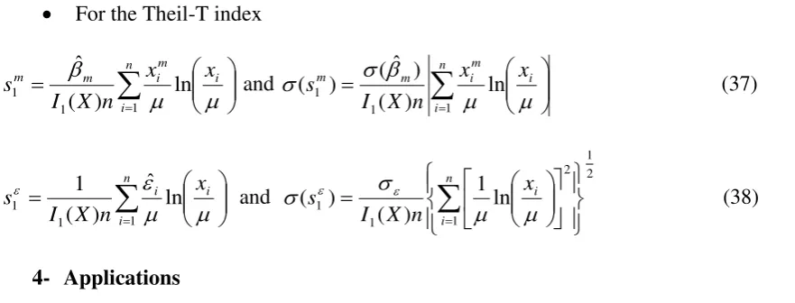
 For the Theil-T index



 

   

 n

i

i m i m

m x x

n X I s

1 1

1 ln

) (

ˆ

  

and



 

   

 n

i

i m i m

m x x

n X I s

1 1

1 ln

) (

) ˆ ( ) (

  



 (37)



 

   

 n

i

i x

n X I s

1 1

1 ln

ˆ ) (

1

  

 _and 2

1

2

1

1 ln

1 )

( ) (

   

   

   

 

     







n

i

x n

X I s

  

   ₍₃₈₎

4- Applications

Illustration From Cameroonian rural Data

Data from the country’s household survey known as ECAM (‘Enquête Camerounaise auprès des ménages’) is used. It is conducted every 5 years by the National Statistical Office in Cameroon. For illustration we consider ECAM II which corresponds to the

year 2001 and we restraint the study to the rural zone of the Centre province of

Cameroon (Povince du centre). The survey provides 390 observations of households

in this rural zone.

Our analysis has two parts. First we begin with the evaluation of the contribution of

various consumption sources to the total consumption inequality. Second, we

introduce the regression-based method to estimate the determinant of the total

consumption (as proxy of the total income) inequality.

3.1- Consumption sources factors decomposition

We decompose the total consumption into nine types of consumption sources. For

every household we have the corresponding consumption source per capita: (a) food

(b) Clothing (c) Housing; (d) House servicing (e) Health (f) Transport and

[image:20.595.71.512.85.253.2]

communication (g) Education (h) Personal Treatment (i) leisure.

Table 1 gives the statistics characteristic of these nine variables. The second column of

the table contains the average share of the total consumption of each consumption

(21)

[image:21.595.96.568.101.300.2]

20

Table 1: Statistic characteristics of consumption sources variables

Consumption

Sources Consumption

share

Coefficient of variation

Share flows by Mean

Min First quartile Second quartile

Third

quartile Max

Food 0,4899 0,9289 0,06 0,51 0,77 1,15 10,54

Clothing 0,0456 1,6386 0,00 0,20 0,52 1,08 14,85

Houses

servicing 0,0450 2,0164 0,00 0,30 0,56 1,06 29,21

Health 0,0956 1,9058 0,00 0,17 0,43 0,89 19,21

Transport 0,0789 2,3077 0,00 0,18 0,42 0,93 26,68

Education 0,0401 2,4618 0,00 0,00 0,23 0,94 26,14

Personnel

care 0,0161 3,2055 0,00 0,17 0,53 1,05 59,27

Leisure 0,0042 3,5923 0,00 0,00 0,00 0,34 32,07

Housing 0,1846 0,9551 0,13 0,46 0,73 1,11 8,41

Total _1,0000 _0,7895 _0,07 _0,53 _0,76 _1,20 _6,49

Source: Own calculation on ECAM II database

We observe that the most important source of consumption is Food which represents

almost 49% of the total consumption. Food is also the consumption source with

relative smaller coefficient of variation but this coefficient of variation is greater than

the total consumption one. In the same spirit, but with lower acuity, we have Housing

and Heath which represent respectively 18.46% and 9.56% share of the total

consumption. Thus we presage important role in total consumption inequality

increases contributions of these variables.

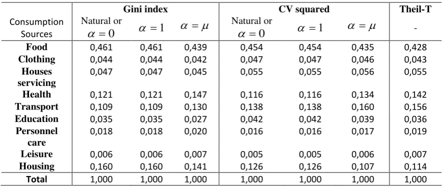
Table 2: Consumption sources contributions to inequality

Gini index CV squared Theil-T

Consumption Sources

Natural or

0 

  1   Natural or  0  1   -

Food 0,461 0,461 0,439 0,454 0,454 0,435 0,428

Clothing 0,044 0,044 0,042 0,047 0,047 0,046 0,043

Houses servicing

0,047 0,047 0,045 0,055 0,055 0,056 0,055

Health 0,121 0,121 0,147 0,116 0,116 0,134 0,142

Transport 0,109 0,109 0,130 0,138 0,138 0,160 0,156

Education 0,035 0,035 0,027 0,042 0,042 0,039 0,036

Personnel care

0,018 0,018 0,020 0,016 0,016 0,017 0,019

Leisure 0,006 0,006 0,007 0,005 0,005 0,006 0,007

Housing 0,160 0,160 0,141 0,126 0,126 0,107 0,114

Total _1,000 _1,000 _1,000 _1,000 _1,000 _1,000 _1,000

Source: Own calculation on ECAM II database

In Table 2, we have computed the inequality contributions of the sources

[image:21.595.100.545.505.693.2]

(22)

21

rules: Gini and CV squared with  0, 1,   , and the natural decomposition of Theil-T index. Notably, the different decomposition methods are concordant. They

assign almost the same amount of contributions to each consumption source. As

noticed, our expectation is satisfied by all the seven decompositions rules. Food

constitutes the most important consumption inequality-increasing source followed

far-off by Housing and Health. In this particular analysis, the difference is not sensitive

between decomposition rules satisfying the uniform additions property and those

which do not satisfy this property. However, this is not a general rule. As we have

already mentioned, this situation will arrive whenever among the consumption

sources, there is none of them with a large average total consumption share, which is

evenly distributed. Particularly, when one of the attributes (or income inequality

determinant) is constant, the effect of the uniform additions may be perceptive. This

will be exemplified with the regression-base model.

3.1 Determinants of the income inequality: The regression-based model

The variables we use to explain per capita income3 (consumption) are listed in the first

column of table 3. We include age of the head of household. We have also used its

squared value to account for life-cycle effect but it was not statistically significant and

was removed from the analysis. We also include a set of binary indicators of the

educational level of the head of household. Household size and composition are

represented by two variables: family size and the fraction of working age in the

family. The working age in the family is taking to be from 20 to 60. The economic

resource of the household is essentially represented by per capita land owned. We also

include a dummy indicator for the household head being a male. Since the Catholic

religion plays a central role in the region, we have included a dummy variable for the

head of the household being catholic. The second column of the table 3 contains the

means of explanatory variables and it reveals that 72.7% of household heads are male

and more than 77% are catholic.

3

(23)

22

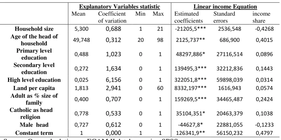
Table 3 :Explanatory Variables and Linear income Generating Equation

Explanatory Variables statistic Linear income Equation

Mean Coefficient of variation

Min Max Estimated coefficients

Standard errors

income share

Household size 5,300 0,688 1 21 -21205,5*** 2536,548 -0,4268

Age of the head of

household 49,748 0,312 20 98 2125,737** 686,900 0,4015 Primary level

education 0,488 1,023 0 1 48297,886* 27116,514 0,0896 Secondary level

education 0,272 1,634 0 1 139495,3*** 32212,836 0,1443 High level education 0,025 6,156 0 1 322051,8*** 59898,039 0,0314

Land per capita 1,813 2,941 0 60 8332,197*** 1616,943 0,0574

Adult as % size of

family 0,400 0,707 0 1 159269,5*** 34465,487 0,2424 Catholic as head

religion 0,778 0,533 0 1 35104,351* 20463,379 0,1038 Male head 0,727 0,612 0 1 -44627,8* 22881,055 -0,1233

Constant term 1 0,000 1 1 126341,9** 56150,232 0,4797

Source: Own calculation on ECAM II database using SPSS program.

***coefficient significant at 1%, **coefficient significant at 5%, *coefficient significant at 10%. R2=0.364and R2adj=0.348.

Dependent variable = Total household Income per capita. Nb observations = 389

Income Inequality Decomposition

The filth column of table 3 gives the coefficient of the linear equation estimated by the

OLS method and the sixth column gives standard errors. Notably, almost all estimated

coefficients are statistically significant ( five of them : Household size , Secondary

level of education, High level of education, Land per capita and Adult as % size of

family are strongly significant at 99% level of confidence) and they have the expected

sign. Household size have a negative effect while the effect of Adult as % size of

family is positive, per capita income decreases with the size of the family but increases

with the Fraction of working-age adults. The three variables accounting for education

each have a positive effect and the impact of these effects increases with the level of

schooling. It is worth noting that the High level education and the Secondary level

education effects are highly significant while the significance of the Primary level

education is lower. This confirms that per capita income increases with the level of

education of household head. Age has a positive effect and male-headed households

have lower income per capita than female-headed households, but the effect of gender

issues is not highly significant. Per capita income increases with Land owned per

[image:23.595.85.544.90.319.2]

(24)

23

catholic religion is relatively low since it is statistically significant only at 90% level

of confidence.

The seventh column corresponds to a measure of the relative magnitude of the effect of the explanatory

variables on the income. It gives average income share

x x_m

m

ˆ _{of each explanatory variable. Note}

that none of the educational variables induces a large share of average income. On the contrary, the

demographic variables such as Household size (negatively), Age and Fraction of working-age adults

present considerable income share. The constant term also plays a substantial role in average income

sharing. Consequently, we expect relatively large influence of these variables on income inequality

[image:24.595.90.586.303.692.2]

contributions.

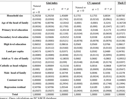
Table 4: Contribution to the income inequality

Gini index CV squared Theil-T

Natural or

0 

  1  

Natural or

0 

  1   -

Household size 0,29258 (0,0350)

0,29258 (0,0350)

1,45689 (0,1743)

0,1755 (0,0210)

0,8034 (0,0961)

0,88700 (0,1061)

Age of the head of family 0,00796 (0,0026)

0,00796 (0,0026)

-0,53542 (0,1730)

-0,0001 (0,000)

-0,3241 (0,1047)

-0,36728 (0,1187)

Primary level education -0,02663 (0,0150)

-0,02663

(0,0150)

-0,20118

(0,1130)

-0,0186

(0,0104)

-0,0186

(0,0104)

-0,1173

(0,0659)

-0,12953

(0,0727)

Secondary level education 0,03606 (0,0083)

0,03606 (0,0083)

-0,05252 (0,0121)

0,0338 (0,0078)

-0,0330 (0,0076)

-0,05963 (0,0138)

High level education 0,06032 (0,0112)

0,06032 (0,0112)

0,08616 (0,0160)

0,0569 (0,0106)

0,0766 (0,0142)

0,08617 (0,0160)

Land per capita 0,04573 (0,0089)

0,04573 (0,0089)

0,01971 (0,0038)

0,0592 (0,0115)

0,0489 (0,0095)

0,04781 (0,0093)

Adult as % size of family 0,07038 (0,0152)

0,07038 (0,0152)

-0,18035 (0,039)

0,0682 (0,0148)

-0,0802 (0,0174)

-0,09552 (0,0207)

Catholic as head religion 0,00004 (0,000)

0,00004 (0,000)

-0,15156 (0,0883)

0,0016 (0,0009)

-0,0868 (0,0506)

-0,09734 (0,0567)

Male head of family 0,00650 (0,0033)

0,00650 (0,0033)

0,16744 (0,0859)

0,0046 (0,0024)

0,1036 (0,0531)

0,12278 (0,0629)

Constant term 0,00000 (0,0000)

0,00000 (0,0000)

-0,66461 (0,2954)

0,0000 (0,0000)

-0,3934 (0,1748)

-0,44865 (0,1994)

Regression residual 0,50706 (0,0507)

0,50706 (0,0507)

1,05544 (0,1660)

0,6189 (0,0404)

1,0024 (0,0908)

1,05420 (0,0926)

Total 1,00000 1,00000 1,00000 1,0000 1,0000 1,0000 1,00000

Source: Own calculation on ECAM II database Standard errors are in parentheses

We now tackle the decomposition of the inequality by income determinants, results

(25)

24

three inequality indices (Gini, CV squared and Theil-T) and the two decomposition

methods (natural decomposition and the proposed alternative method). Notably, the

seven decomposition rules in table 4, in term of similarity of the sign and the

contribution amount assigned to each income determinant, can be subdivided into two

homogeneity groups. The first group is composed by the natural decomposition

(or 0)of the Gini and the CV squared indices and the alternative decomposition of these indices with  1. The second group consists of the alternative decomposition method of the Gini, the squared CV with  and the Theil-T index natural

decomposition. This clearly demonstrates the effect of the parameter  on the alternative method in one hand and the impact of the uniform addition property to the

inequality decomposition in the other hand. Note that the alternative decomposition

methods for Gini and the alternative decomposition for CV squared indices with  1

satisfy the uniform additions property but the weight of parameter  is too light to capturethe influence of the second term (see Eq.11 and Eq.19b) of the decomposition

rule.Thus, these two decompositions rule practically assigned the same contribution to

every variable as their respective natural decomposition; this is no surprise.According

to the first group of decompositions methods, the constant term contributes nothing to

the inequality. While Household Size constitutes the major contributor to

inequality-increasing, followed far away by Fraction of working-age adults. All four

decomposition rules of this group assign little amount to the education variables. We

note that, here, Primary level education acts to reduce inequality, but only by about

2%. Except the null contribution of the constant term which represents a considerable

share of average income, these results are not very far from our expectation as

mentioned above. However, it is surprising that Age of head of household, which has

an important role in explaining income and which average income share is relatively

large, has a much smaller income inequality contribution.

All decomposition rules in the second group assign the same sign and the same level

of amount to proportional contribution of each variable. This, in particular, shows that

the alternative Gini decomposition rule with neatly agree with the Theil-T

(26)

25

squared4 (Morduch and Sicular (2002)). Consider now the variables Household size,

Age and Fraction of working-age adults. Each of them has a large income average

share and they are relatively evenly distributed (see table 3). As expected, the three

decomposition rules give a substantial inequality reduction for Age and Fraction of

working-age adults as inequality increases for Household size. A similar observation

holds for Catholic households headed and Male households headed but with a little

less acuity. The Catholic religion reduces inequality while being a male

household-head operates to increase inequality. Of course, the constant term contributes toward

reducibly inequality and we note that this reduction is little more important with the

Gini alternative decomposition than the others decomposition methods of the group.

The two groups of decomposition methods give each a positive contribution to the

Regression residual with more importance in the second group5. This gap can be, in

part, explained by the compensation due to the negativity of the constant term

contribution when the uniform addition property holds.

5- Concluding remarks

The paper has provided a new factor decomposition rules for classical inequality

indices such as Gini index and the squared coefficient of variation. From the onset it

was presumed that the decomposition rule must satisfy the uniform additions property.

The approach adopted consists in adding a corrective term to the natural Shorrocks

decomposition formula. We have obtained a parametric family of decomposition rules

with several basic properties conserved and which make it an attractive family of

decompositions procedures. The parameter of the decomposition family, which is

defined as a real function of the total income can be seen as a bridge between the

natural decomposition, which satisfy normalization axiom, and the others members of

family which satisfy uniform additions property. It is important to point out that the

impact of the uniform addition property in the decomposition rule is in proportion with

the magnitude of the parameter value chosen. This brings out the natural question of

4

It is no surprise that the alternative decomposition rule of the CV squared (with  ) being in concordance with the natural decomposition of the Theil-T index. As we have already mentioned, the former coincides with the natural decomposition of the entropy index with  2 while the latteris the natural decomposition of the entropy index with 1.

5