Spreading Dynamics of a Social Information Model with Overlapping Community Structures on Complex Networks

(1)

How to cite this paper: Liu, X.D., Li, T., Wang, Y.M. and Wan, C. (2016) Spreading Dynamics of a Social Information Model with Overlapping Community Structures on Complex Networks. Open Access Library Journal, 3: e2701.

http://dx.doi.org/10.4236/oalib.1102701

Spreading Dynamics of a Social Information

Model with Overlapping Community

Structures on Complex Networks

Xiongding Liu, Tao Li

*

_{, Yuanmei Wang, Chen Wan}

School of Electronics and Information, Yangtze University, Jingzhou, China

Received 30 April 2016; accepted 27 May 2016; published 30 May 2016

This work is licensed under the Creative Commons Attribution International License (CC BY). http://creativecommons.org/licenses/by/4.0/

Abstract

In this paper, we present a SARS (susceptible-adopted-removed-susceptible) social information spreading model with overlapping community structures on complex networks. Using the mean field theory, the spreading dynamic of the model has been studied. At first, we derived the spreading critical threshold value and equilibriums. Theoretical results indicate that the existence of equilibriums is determined by threshold value. The threshold value is obviously dependent on the topology of underlying networks. Furthermore, the globally asymptotically stable equili-briums are proved in detail. The overlap parameter of community structures can't change the threshold value, but it can influence the extent of the social information spreading. Numerical si-mulations confirmed the analytical results.

Keywords

Social Information Spreading, Overlap Parameter, Community Structures, Complex Networks, Threshold Value

Subject Areas: Network Modeling and Simulation

1. Introduction

Complex networks can be described by many real-world systems [1]-[3], in which nodes represent individuals while edges represent the relationships or interactions between nodes. Examples include social information net-works [4]. Social information networks offer a diverse range of possible group organizations, such as relation-ship, communication and friendship circles. Some experiments on several networks with ground-truth groups and temporal attributes reveal that two nodes are likely to be connected if some of their neighbor nodes are in the same communities [5]. L.J. Zhao and J.J. Wang found that the dynamic behavior of rumor spreading is based

(2)

OALibJ | DOI:10.4236/oalib.1102701 2 May 2016 | Volume 3 | e2701

on the SIR (susceptible-infected-recovered) epidemic spreading model [6]. The DK and MK models have been used comprehensively for quantitative studies of rumor spreading [7]-[13], but the major deficiencies of these models are that they have not considered the topological characteristics of overlapping community structure for describing rumor spreading in social networks.

With the study of network structural properties, the spread of an epidemic over complex networks has inves-tigated very mature [14]-[16]. A SIQRS (susceptible-infected-quarantined-recovered-susceptible) epidemic model on scale-free network investigates the influence of heterogeneity of the underlying networks and quarantine strategy on epidemic spreading [17]. Pastor-Satorras and Vespignani set the absence of a SIS (susceptible-infected-susceptible) epidemiological model on the infinite scale-free network [18]. In addition, SIS spreading on scale-free networks with degree correlations has also been proved [19]. Besides, a SEIRS (susceptible-exposed- infected-recovered-susceptible) model with infectivity assumed to be either constant or proportional to the node degree on scale-free networks was presented in [20]. These models—the local stability analysis of the disease- free equilibrium and the permanence of the disease in the network, were provided and proved.In the reference

[21], it has presented four real networks for both SIR and SI spreading models; the DS centrality is more precise than degree.

In sum, the rumor or disease transmission model contributes to understanding the intrinsic mechanisms of those spreading processes and designing efficient control strategies. However, information spreading has differ-ence from disease infections because of its specific features, such as time decaying infludiffer-ence [22], the link of nodes degree [23], information contents [24], effects of memory [25], social stabilize [26] [27], non-redundancy of contacts [28], etc. In this paper, we present a new model SARS to illustrate social information spreading on overlapping community structures. It has assumed a novel generative model and formalized the detection of overlapping communities as well as hubs as an optimization problem on it [29]. We propose each community in an oblivious way. That is, considering the membership of a node may belong to more than one community, and we do not care whether it has been already allotted to any communities. Overlapping communities are thus na-turally supported. In the centrality matrix, a node ranked at the top of the community is seen as a center. There-fore, regardless of the fact that the number of communities is given or not, the method that we proposed is capa-ble of detecting overlapping communities as well as hubs simultaneously.

In Section 2, we present a SARS social information spreading model with overlapping community structures and introduces related work on complex networks. In Section 3, we analyze the globally asymptotically stable equilibriums in detail. In Section 4, numerical experiments and simulation results are given to illustrate the theoretical results. Finally, conclusions and future works are drawn in Section 5.

2. Model Formulation

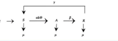
In this article, we discussed the social information spreading on complex networks with the overlapping com-munity structure. Overlapping comcom-munity structure is mainly to describe the network topology relatively strongly linked to the internal part of the node and the external characteristic of contact relatively sparse. We use a SARS model to illustrate the proposed social information spreading process. In this model, we assume that so-cial information spreading is disseminated by direct contacts of adopted nodes with others, and the population is divided into three groups: susceptible (S), adopted (A), removed (R), where S, A, R represent the people who never heard the information (Susceptible), those who are spreading information (Adopted), and the ones who heard the information but have lost interest in diffusing it (Removed). From now on, we refer to the SARS model as the information spreading model. On the size of the N in the social information network, we suppose there are two communities with the same size A and B. We defined v is an overlap parameter. The probability of each adopted nodes connect to any node in the community A by v, with the probability of 1−v to the community B. On the edge of the process we do not allow the existence with the heavy side. Due to the symmetry between community A and B, so we take v∈

(

0.5,1

)

. A large number of experiments show that the social information network is a sparse network. In the course of social information spreading, a susceptible individuals is infected with rate α if it is connected to an adopted individuals. Due to the invalidation and distortion of social infor-mation the adopted individuals will change to removed individuals by β . However, some removed individual because temporary amnesia will join susceptible individuals again with probability γ. Here, we assume that the immigration rate l equals the emigration rate µ. The SARS model has the flow diagram given in Figure 1 with the above assumptions.

(3)

[image:3.595.239.444.85.156.2]

OALibJ | DOI:10.4236/oalib.1102701 3 May 2016 | Volume 3 | e2701 Figure 1. The flow diagram of the SARS model.

vertices with different connectivity, let S t_k

( )

, A t_k

( )

and R t_k

( )

be the relative densities of susceptible, adopted and removed nodes of degree k at time t respectively. With these signs and symbols, the dynamics mean-field reaction rate equations can be written as

( )

_{( )}

_{( ) ( )}

_{( )}

( )

_{( ) ( )}

_{( )}

( )

_{( )}

d d d d d d k

k k k

k

k k k

k

k k k

S t

l R t k t S t S t

t A t

k t S t A t A t

t R t

A t R t R t

t

γ α µ

α β µ

β γ µ



= + − Θ −

  

= Θ − −

   = − −   (2.1)

The dynamics of SARS subsystems are coupled through the function Θ

( )

t . The probability Θ

( )

t describes a link pointing to an adopted individual. Which satisfies

( )

t v A

( ) (

t 1 v

) ( )

B t

Θ = Θ + − Θ ,

where

( )

1

( )

Ak k

A Ak

k s

kP k A t

k kP k A t

sP s

−

Θ =

∑

=

∑

;

( )

1

( )

Bk k

B Bk

k s

kP k A t

k kP k A t

sP s

−

Θ =

∑

=

∑

.

So

( )

1

( )

( ) (

)

1

( )

1

Ak Bk

k k

t v k − kP k A t v k − kP k A t

Θ =

∑

+ −

∑

(2.2)

where P k

( )

>0 is the probability that a node has degree k and thus

( )

1 1

n

k= P k =

∑

;

( )

1 n k

k =

∑

₌kP k de-notes the average degree [30].

( )

( ) ( )

1 n

k k

A t =

∑

₌ P k A t is the total density of adopted individuals in the net-work. Clearly, these variables obey the normalization condition: S_k

( )

t +A t_k

( )

+R t_k

( )

=1. The initial condi-tions for system (2.1) can be given as follows S_k

( )

0 = −1 A_k

( )

0 −R_k

( )

0 >0,A_k

( )

0 ≥0,R_k

( )

0 ≥0.

Definition. The equilibrium is an information-free equilibrium if A=0.

Theorem 1. Let

2 c k k α λ β µ =

+ . The SARS system (2.1) has always exists an information-free equilibrium

(

)

0

1,0,0

E and when λ >c 1, then the system (2.1) has a unique permanent equilibrium E

(

Sk,A Rk, k

)

∗ ∗ ∗ ∗ .

Proof. To get the equilibrium solution E∗

(

S_k∗,A R_k∗, _k∗

)

, it should satisfy

( ) ( )

( )

0 0 1

k k k

k t S t A t A t

A t R t R t

S t A t R t

α β µ

β γ µ

∗ ∗ ∗

 Θ − − =

 ₋ ₋ ₌



 ₊ ₊ ₌



(2.3)

This leads to

(

)(

)

(

) (

)(

)

(

)

(

) (

)(

)

(

) (

)(

)

k k k S k k A k k R k

β µ γ µ

α β γ µ β µ γ µ

γ µ α

βα

∗ ∗ ∗ ∗ ∗ ∗ ∗ ∗ + +  =

 _Θ _{+ +} ₊ ₊ ₊



 ₊ _Θ

 ₌

 _Θ _{+ +} ₊ ₊ ₊



 _Θ

 =

Θ + + + + +



(4)

Substituting (2.4) Ak

∗

into (2.2), we obtain that

( )

(

)

(

)

(

)

(

)

(

) (

)(

)

( )

1 1 1 A B

k _A _B

k v v

kP k f

k k v v

γ µ α

∗ ∗

+ Θ + − Θ

Θ = = Θ

Θ + − Θ + + + + +

∑

(2.5)

Clearly, Θ ≥ Θ ≥A 0, B 0, 0

∗

Θ = is a solution of (2.5), at that time Θ =∗_A 0 and Θ =∗_B 0. To ensure (2.5) has a nontrivial solution of f

( )

Θ =0, it must be satisfied as following:

( )

2

0 d 1 d c f k k α λ β µ ∗ ∗ ∗ Θ = Θ

= = >

+

Θ and f

( )

1 ≤1

We can obtain the threshold value:

2 c k k α λ β µ = +

where 2 2

( )

1 n k

k =

∑

₌ k P k . So a nontrivial solution of f

( )

Θ =0 exists if and only if f

( )

1 ≤1, that is ,

1

c

λ > . It follows from (2.3) that (2.4) hold and for k=1, 2,,n, 0 Sk 1, 0 Ak 1, 0 Rk 1.

∗ ∗ ∗

< < < < < <

Hence the system (2.1) has an permanent equilibrium E∗. This completes the proof.

3. The Stability Analysis

In this section, the globally asymptotically stable E0

(

1,0,0

)

and E∗

(

S_k∗,A R_k∗, _k∗

)

will be investigated. We first consider the local asymptotic stability and then the global attractivity of the information-free equilibrium E0. More specifically, we will show that if the threshold value λ <c 1, then

0

E is globally asymptotically stable. Otherwise, it is unstable. We now state the results of the local stability of E0.

Theorem 2. The information-free equilibrium E0 of SARS system (2.1) is globally asymptotically stable if

1.

c

λ <

Proof. First, we prove that E0 is locally asymptotically stable. We rewrite system (2.1) as

( )

₍

_{( ) (}

₎

_{( )}

₎

_{( )}

( )

_{( )}

d 1 d d d k

Ak Bk k k k

k

k k k

A t

k v t v t S t A t A t

t R t

A t R t R t

t

α β µ

β γ µ



= Θ + − Θ − −

 

 ₌ ₋ ₋



(3.1)

After the linearization, we write the system (3.1) as

( )

_{( ) ( )}

_{( )}

( )

_{( )}

d d d d k

Ak k k k k

k k k

A t

v k t S t A t A t

t R t

A t R t R t

t

α β µ

β γ µ

 ₌ _Θ ₋ ₋

 

 ₌ ₋ ₋



(3.2)

Then the Jacobian matrix of (3.2) at E0 is given by

1 12 13

2

1 2 3 2 2

n n n n n n

M N N N

N M N N

J

N N N M _×

      =_ _             where

( ) (

)

2 1 0 j

v k P k k

M α β µ

β γ µ

(5)

( )

2 1 0 0 0 ij

v k P k k N α     =      

Using induction on n, the characteristic equation can be expressed as

(

)

(

)

(

)

1

(

)

2

( )

0

n n v k P k

x x x

k

α

µ γ β µ −  β µ 

+ + + + _ + + − _=

  (3.3)

The characteristic equation have n eigenvalues for − − <

λ µ

0, n−1 eigenvalues equal to −

(

β µ

+

)

<0, the 2nth eigenvalue is

( )

₍

₎₍

₎

2

1

c v k P k

v k

α _{β µ} _{β µ} _λ

− − = + − . Since 2 1 c k k α λ β

= < and 0< ≤v 1, so vλ_c≤λ_c,

(

)

(

)

1

1 0

n

k k c

k

A B

β µ

v

λ

=

− − = + − <

∑

.

All the eigenvalues of J are negative if λ <c 1. Hence,

0

E is locally asymptotically stable and it is unstable if λ >c 1. This completes the proof.

Next, we will prove that the equilibrium E0 is indeed globally attractive. From the second equation of sys-tem (2.1) we have

( )

_{( )}

₍

_{( ) (}

₎

_{( )}

₎

_{( )}

( )

( ) (

)

( )

(

)

( )

(

)(

)

( )

1 1 2

d 1 1

1 d

1

n

Ak Bk k k k

k k n k Ak k Ak c Ak t

kP k k v t v t S t A t A t

t k k

kP k kS t t

k

t k

t

α β µ

α µ β

α

µ β

µ β λ =

= Θ

 

= _ Θ + − Θ − − _

 

≤_ − + _Θ

 

 

 

< − + Θ

 

 

= + − Θ

∑ ∑

∑

Now we consider the comparison equation with the condition Θ

( )

0 =

ϕ

( )

0 as follows:

( ) (

) ( )(

)

d 1 d c t t t

ϕ _{µ β ϕ} _λ

= + −

Integrating from 0 to t yields, ϕ

( )

_t =ϕ

( )

0 e(µ β λ+ )(c−1)t_{, Since} ₁ c

λ < , we have

ϕ

( )

t →0 as t→ ∞.

According to the comparison theorem of functional differential equation, we have 0≤ Θ

( )

t ≤

ϕ

( )

t , for all 0

t> .

Therefore, Θ

( )

t →0 as t→ ∞, which means A tk

( )

→0 as t→ ∞, for k=1, 2,,n. It follows that

the information-free equilibrium E0 is globally attractive. Hence, E0 is locally asymptotically stable if

1

c

λ < and it is unstable if λ >c 1. This completes the proof.

We now prove the globally asymptotically stable of equilibrium E∗ of SARS system (2.1).

Theorem 3. When λ >c 1, the information spreading is persistence on the scale-free networks, there exists a 0

ς

> , such that

( )

( ) ( )

lim inf lim inf k

x x

k

A t P k A t ς

→∞ = →∞

∑

>

(6)

(

)

{

1, 1, 1, , kmax, kmax, kmax : k, k, k 0 and k k k 1, 1, , max

}

, X = S A R  S A R S A R ≥ S +A +R = k=  k

(

max max max

)

( )

0 1, 1, 1, , k , k , k : k 0 , k

X = S A R S A R ∈X P k A > 

 

∑



0 \ 0

X X X

∂ =

Obviously, X is positively invariant with respect to system (2.1). If Sk

( )

0 ≥0,

( )

k 0 k

P k A >

∑

and Rk

( )

0 ≥0

for k=1,,k_max, then Sk

( )

0 ≥0,

( )

k 0 k

P k A >

∑

and Rk

( )

0 ≥0 for all t>0. Since

( ) ( )

k

(

)

( ) ( )

k

k k

P k A t µ β P k A t

′

 _{ ≥ − +}

 



∑



∑

and

( ) ( )

k 0 0

k

P k A >

∑

, we have

( ) ( )

( )

0 e t 0

k k

P k A t ≥ P k A − +µ β >

∑

. Thus, X₀ is also positively invariant. Furthermore, there exists a compact set Y in which all solutions of system (2.1) initiated in X will enter and remain forever after. The com-pactness condition (C4.2) in Thieme [32] is easily proved for this set Y. Denote

( ) ( ) ( )

( )

(

)

{

( ) ( ) ( )

( )

(

)

}

max max max

1 1 1

1 1 1 0

0 , 0 , 0 , , 0 , 0 , 0 :

, , , , , , , 0 .

k k k

M S A R S A R

S t A t R t S t A t R t X t

∂ = ∈ ∂ ≥  

( ) ( ) ( )

( )

(

)

{

( ) ( ) ( )

( )

(

)

}

max max max

1 1 1

0 , 0 , 0 , , 0 , 0 , 0 :

0 , 0 , 0 , , 0 , 0 , 0 ,

k k k

S A R S A R

S A R S A R X

ω Ω = ∪

∈



where

(

( ) ( ) ( )

( )

)

max max max

1 0 , 1 0 , 1 0 , , k 0 , k 0 , k 0

S A R S A R

ω _ is the omega limit set of the solutions of system

(2.1) starting in

(

( ) ( ) ( )

( )

)

max max max

1 0 , 1 0 , 1 0 , , k 0 , k 0 , k 0

S A R  S A R , Restricting system (2.1) on M∂ gives

( )

_{( )}

( )

_{( )}

( )

_{( )}

d d d d d d k k k k k k k k k S t

l R t S t

t A t

A t A t

t R t

R t R t

t γ µ µ β γ µ  _{= +} ₋    _{= −} ₋    = − −   (3.4)

It is easy to verify that system (3.4) has a unique equilibrium E0 in X. Thus E0 is the unique equilibrium of system (2.1) in M∂. It is easy to demonstrate that E0 is locally asymptotically stable. This means that E0

is globally asymptotically stable for (3.4) is a linear system. Therefore Ω =

{ }

_E0 _{. And} 0

E is a covering of X, which is isolated and is acyclic (since there exists no solution in M∂ which links E0 to itself). Finally, the

proof will be done if we show E0 is a weak repeller for X₀,

( ) ( ) ( )

( )

(

)

(

max max max

)

0

1 1 1

lim sup , , , , k , k , k , 0

t→∞ dist S t A t R t  S t A t R t E >

,

where

(

( ) ( ) ( )

( )

)

max max max

1 , 1 , 1 , , k , k , k

S t A t R t  S t A t R t is an arbitrarily solution with initial value in X₀. By Leenheer and Smith [31], we need only to prove

( )

0

0 s

W E ∩X = ∅ where _Ws

( )

_E0 _{is the stable mani-}

fold of E0. Suppose it is not true, then there exists a solution

(

( ) ( ) ( )

( )

)

max max max

1 , 1 , 1 , , k , k , k

S t A t R t  S t A t R t

in X₀, such that

( )

1,

k

(7)

OALibJ | DOI:10.4236/oalib.1102701 7 May 2016 | Volume 3 | e2701 Since 2 1 c k k α λ β µ = >

+ , we can choose

η

>0, such that

(

)

2

1 1 c k k α η λ β µ − = > + .

For

η

>0, by (3.5) there exists a T >0 such that

( )

1− <

η

Sk t < +1

η

, 0≤A tk <

η

, 0≤R tk <

η

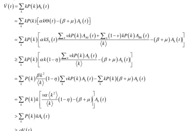
for all t≥T and k=1,,k_max. Let

( )

( ) ( )

k k

V t =

∑

kP k A t .

V represent the proportion of all adopted individuals to all individuals. The derivative of V along the solution of system (2.1) is given by

( )

( ) ( )

( ) (

) ( )

( )

(

) ( )

( ) (

) ( )

( )

(

)

( ) ( ) (

) ( )

( )

(

)

( ) ( )

( )(

) ( )

( )

(

) (

) ( )

( )

2 2 ( ) 1 1 1 1 k k k k Ak Bk k k k k k k k k k k k

k k k

k k

V t kP k A t

kP k k t A t

vkP k A t v kP k A t

kP k kS t A t

k

vkP k A t

kP k k A t

k

P k vkP k A t kP k A t

k

v k

P k k A t

k

P k kA t

V t

α β µ

α η β µ

β _η _{β µ}

α

η β µ

ρ =

= _ Θ − + _

 + −  = _ − + _     ≥  − − +    = − − +     = − − +     > ≥

∑



There

ρ

→0+. Hence V t

( )

→ ∞ as t→ ∞, which contradicts to the boundedness of V t

( )

. This completes the proof.

4. Numerical Simulation

In this section, we will give some numerical simulations to illustrate the theoretical analysis. We consider the system (2.1) on a scale-free network with the degree distribution P k

( )

=

ξ

k−3, where the parameter

ξ

satis-fies 3

1 1

n k ξk

−

= =

∑

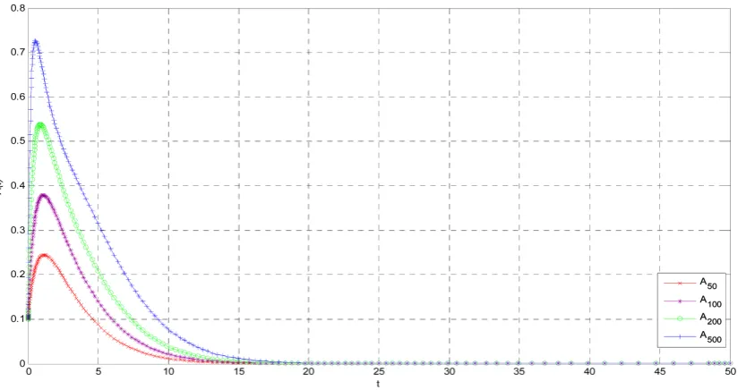
, we choose n=1000.

In Figure 2, we choose α =0.15,l=0.2,µ=0.2,γ =0.6,β =0.5,v=1, thus the threshold value R0=0.9757 1

< . The figure show that when R0 <1, A_k approach to zero, the social information spreading will ultimately disappear, and the smaller the degree is, the faster the social information spreading fades out. It also suggests that the information-free equilibrium E0 is globally asymptotically stable.

[image:7.595.133.506.265.520.2]

(8)

[image:8.595.110.527.84.302.2]

OALibJ | DOI:10.4236/oalib.1102701 8 May 2016 | Volume 3 | e2701 Figure 2. The time series and orbits of system (4) with _R0<₁_{and initial values}

( )

0 0.1, 50, 100, 200, 500.

k

[image:8.595.95.534.335.580.2]

A = k=

Figure 3. The time series and orbits of system (2.1) with 0

1

R > and initial values A_k

( )

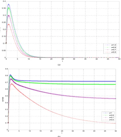
0 =0.1, k=50, 100, 200, 500.

In Figure 4(a), the parameters are α=0.15,l=0.2,µ=0.2,γ =0.6,β =0.5, R0=0.9757. Likewise, we choose α=0.5,l=0.2,µ=0.4,γ =0.6,β=0.4 in Figure 4(b), where R0 =2.84. This two figure shows that the corresponding A₁₀₀ increases significantly as the overlap parameter v increase. In addition, it is also found that the larger overlap parameter is, the higher the social information spreading level will be. The biological meaning is that the closer overlapping communities is, the wider social information spreading will be, corres-ponding to people’s frequency with each other.

(9)

(a)

[image:9.595.112.523.86.553.2]

(b)

Figure 4. The prevalence A₁₀₀ versus t corresponding to different v, which are 0.5, 0.7, 0.9, 1 from (a) to (b), with iden-tical initial value A₁₀₀

( )

0 =0.1.

5. Conclusion

(10)

[image:10.595.94.542.85.342.2]

OALibJ | DOI:10.4236/oalib.1102701 10 May 2016 | Volume 3 | e2701 Figure 5. The prevalence A

( )

100 versus v corresponding to different β, β=0.4 or 0.7.

Acknowledgements

This work was supported in part by the National Natural Science Foundation of China under Grants 60973012, 6147234.

References

[1] Strogatz, S.H. (2001) Exploring Complex Networks. Nature, 410, 268-276. http://dx.doi.org/10.1038/35065725

[2] Albert, R. and Barabási, A.-L. (2002) Statistical Mechanics of Complex Networks. Reviews of Modern Physics, 74, 47-

97. http://dx.doi.org/10.1103/RevModPhys.74.47

[3] Newman, M.E.J. (2003) The Structure and Function of Complex Networks. SIAM Review, 45, 167-256.

http://dx.doi.org/10.1137/S003614450342480

[4] Wasserman, S. (1994) Social Network Analysis: Methods and Applications. Vol. 8. Cambridge University Press, Cambridge. http://dx.doi.org/10.1017/CBO9780511815478

[5] Dowling, J.E. (2002) Proceedings of the National Academy of Sciences of the United States of America. Nutrition Re-views, 99, 7821.

[6] Zhao, L.J. and Wang, J.J. (2012) SIHR Rumor Spreading Model in Social Networks. Physica A, 391, 2444-2453.

http://dx.doi.org/10.1016/j.physa.2011.12.008

[7] Newman, M.E.J. and Forest, S. (2002) Email Networks and the Spread of Viruses. Physical Review E, 66, Article ID: 035101.

[8] Smith, R.D. (2002) Instant Messaging as a Scale-Free Network. arXiv preprint cond-mat, 0206378..

[9] Csanyi, G. and Szendroi, B. (2004) Structure of a Large Social Networks. Physical Review E, 69, Article ID: 036131.

http://dx.doi.org/10.1103/physreve.69.036131

[10] Wang, F. and Moreno, Y. (2006) Structure of Peer-To-Peer Social Network. Physical Review E, 73, Article ID: 036123.

http://dx.doi.org/10.1103/physreve.73.036123

[11] Pittel, B. (1990) On a Daley-Kendall Model of Random Rumours. Journal of Applied Probability, 27, 14-27.

http://dx.doi.org/10.2307/3214592

[12] Lefevre, C. and Picard, P. (1994) Distribution of the Final Extent of a Rumor Process. Journal of Applied Probability,

(11)

OALibJ | DOI:10.4236/oalib.1102701 11 May 2016 | Volume 3 | e2701 [13] Gu, J. and Li, W. (2008) The Effect of the Forget-Remember Mechanism on Spreading. The European Physical

Jour-nal B, 62, 247-255. http://dx.doi.org/10.1140/epjb/e2008-00139-4

[14] Draief, M. (2006) Epidemic Processes on Complex Networks. Physica A, 363, 120-131.

[15] Wang, J. (2007) Epidemic Spreading on Uncorrelated Heterogenous Networks with Non-Uniform Transmission. Phy-sica A, 382, 715-721. http://dx.doi.org/10.1016/j.physa.2007.04.034

[16] Peng, C., Jin, X. and Shi, M. (2010) Epidemic Threshold and Immunization on Generalized Networks. Physica A: Sta-tistical Mechanics and Its Applications, 389, 549-560. http://dx.doi.org/10.1016/j.physa.2009.09.047

[17] Li, T., Wang, Y.M. and Guan, Z.-H. (2014) Spreading Dynamics of a SIQRS Epidemic Model on Scale-Free Networks.

Communications in Nonlinear Science and Numerical Simulation, 19, 686-692.

http://dx.doi.org/10.1016/j.cnsns.2013.07.010

[18] Pastor-Satorras, R. and Vespignani, A. (2001) Epidemic Spreading in Scale-Free Networks. Physical Review Letters,

86, 3200. http://dx.doi.org/10.1103/PhysRevLett.86.3200

[19] Boguñá, M., Pastor-Satorras, R. and Vespignani, A. (2003) Absence of Epidemic Threshold in Scale-Free Networks with Degree Correlations. Physical Review Letters, 90, Article ID: 28701.

http://dx.doi.org/10.1103/PhysRevLett.90.028701

[20] Liu, J. and Zhang, T. (2011) Epidemic Spreading of an SEIRS Model in Scale-Free Networks. Communications in Nonlinear Science and Numerical Simulation, 16, 3375-3384. http://dx.doi.org/10.1016/j.cnsns.2010.11.019

[21] Liu, J.-G., Lin, J.-H., Guo, Q. and Zhou, T. (2016) Locating Influential Nodes via Dynamics-Sensitive Centrality.

Scientific Reports, 6, Article No. 21380. http://dx.doi.org/10.1038/srep21380

[22] Wu, F. and Huberman, B.A. (2007) Novelty and Collective Attention. Proceedings of the National Academy of Sciences of the United States of America, 104, 17599-17601. http://dx.doi.org/10.1073/pnas.0704916104

[23] Miritello, G., Moro, E. and Lara, R. (2011) Dynamical Strength of Social Ties in Information Spreading. Physical Re-view E, 83, Article ID: 045102. http://dx.doi.org/10.1103/PhysRevE.83.045102

[24] Crane, R. and Sornette, D. (2008) Robust Dynamic Classes Revealed by Measuring the Response Function of Social System. Proceedings of the National Academy of Sciences of the United States of America, 105, 15649-15653.

http://dx.doi.org/10.1073/pnas.0803685105

[25] Dodds, P.S. and Watts, D.J. (2004) Universal Behavior in a Generalized Model of Contagion. Physical Review Letters,

92, Article ID: 218701. http://dx.doi.org/10.1103/PhysRevLett.92.218701

[26] Medo, M., Zhang, Y.C. andZhou, T. (2009) Adaptive Model for Recommendation of News. EPL (Europhysics Let-ters), 88, Article ID: 38005. http://dx.doi.org/10.1209/0295-5075/88/38005

[27] Cimini, G., Medo, M., Zhou, T., Wei, D. and Zhang, Y.-C. (2011) Heterogeneity, Quality, and Reputation in an Adap-tive Recommendation Model. The European Physical Journal B, 80, 201-208.

http://dx.doi.org/10.1140/epjb/e2010-10716-5

[28] Lü, L.Y., Chen, D.B. and Zhou, T. (2011) The Small World Yields the Most Effective Information Spreading. New Journal of Physics, 13, Article ID: 123005. http://dx.doi.org/10.1088/1367-2630/13/12/123005

[29] Wang, X., Cao, X.C., Jin, D., Cao, Y.X. and He, D.X. (2016) The (Un)supervised NMF Methods for Discovering Overlapping Communities as Well as Hubs and Outliers in Networks. Physica A: Statistical Mechanics and Its Appli-cations, 446, 22-34. http://dx.doi.org/10.1016/j.physa.2015.11.016

[30] Li, T., Liu, X.D., Wu, J., Wan, C., Guan, Z.-H. and Wang, Y.M. (2016) An Epidemic Spreading Model on Adaptive Scale-Free Networks with Feedback Mechanism. Physica A: Statistical Mechanics and Its Applications, 450, 649-656.

[31] Thieme, H.R. (1993) Persistence under Relaxed Point-Dissipativity (with Application to an Endemic Model). SIAM Journal on Mathematical Analysis, 24, 407-435. http://dx.doi.org/10.1137/0524026

[32] Smith, H.L. and De Leenheer, P. (2003) Virus Dynamics: A Global Analysis. SIAM Journal on Mathematical Analysis,