Support Vector Machine for Classify Dynamic Human/Vehicle Shapes
Razali M.T
1and Adznan Jantan
11Dept. of Mechatronicr & Robotic Engineering
Faculty of Electrical & Electronic Engineering Universiti Tun Hussein Onn Malaysia
86400 Parit Raja Batu Pahat, Johor
2Dept. of Computer & Communication Engineering
Faculty of Engineering Universiti Putra Malaysia
43400 Serdang, Selangor
1[email protected],2[email protected]
Abstract
Currently Support Vector Machines (SVM) became subject of interest because of its ability to give high classification performance in a wide area of application. Most of the classifier model especially based on supervised learning involve complicated learning model and yet the performance sometimes worst. This paper proposes a SVM model to classify between human and vehicle shapes in various pose. SVM classify data by first construct a decision surface that maximizes the margin between the data. For testing new data, SVM will calculate the sign signifying where this new data reside in the constructed decision surface. The developed model will be used to classify an outdoor scene of human and vehicle shapes in dynamic pose. Results of the experiments showed a satisfied performance with the proposed approach.
1.
I
NTRODUCTIONObject recognition and classification is the sequence of steps that must be performed after appropriate features have been detected. Based on the detected features in an image, one must formulate hypotheses about possible objects in the image. These hypotheses must be verified using models of objects. Not all object recognition techniques require strong hypothesis formation and verification steps. Most recognition strategies have evolved to combine these steps in varying amounts. In the following, a few basic recognition strategies used for recognition objects in different situations are reviewed.
One of the earliest approaches to object recognition is based on template matching. This method based on the concept of finding the similarity between two entities such as points, curves, or shapes
of the same type. In template matching, a template typically a 2D shape of the pattern to be recognized is available. The pattern to be recognized is matched against the stored template while taking into account all allowable pose such as translation and rotation and scale changes. The similarity measurement is normally defined as a metric distance. Various distance measures have been exploited in object include city block distance, Euclidean distance, cosine distance, histogram intersection distance, χ2 statistics distance, quadratic distance, and Mahalanobis distance [1].
Nearest Neighbourhood (NN) classifier [2] is based on the fact that if two elements are close in their representation space, they probably belong to the same class. The nearest neighbour classifier is useful when the number of training samples is small. Each form is represented by a feature vector which represents variance of motion and variance of compactness in a multi-dimensional representation space. In order to identify the class of a form, the form class of its nearest points in the representation space is significant information. A strict rule is to impose that the nearest neighbours belongs to the same class to take a decision. This rule reduces the number of errors, but it leads to many rejects. It can be smoothed by weighting the voting of each neighbour according to its rank or distance.
the net may learn the classification boundaries in its feature space. The most commonly used family of neural networks for recognizing system is the feed-forward network, which includes Multilayer Perceptron (MLP) networks [3].
Support vector machine (SVM) are receiving increasing attention these day and have achieved very good accuracy in pattern recognition. In a binary classification, SVM try to find a hyperplane to separate the data into two classes. In the case in which all the data are well separated, the margin is defined as two times the distance between the hyperplane with the largest margin, which provides good generalization ability based on Vapnik’s VC dimension theory [4]. To increase the classification ability, SVMs first map the data into a higher dimension feature space with kernel function, then use a hyperplane in that feature space to separate the data. For testing a new unseen dataset, SVM calculate the distance of this sample from the decision surface, and produced a sign signifying which side of the surface they reside. SVMs have demonstrated good generalization performance in face recognition [5], plankton recognition [6], gene classification [7], Chinese character classification [8], and text categorization [9].
Recognition techniques are mandatory to add to monitoring system to understand the behaviour of dynamic events in complex scenarios. Template matching and nearest neighbour method capable to classify the object with high accuracy if the data is separable, but if the data is in non separable case, neural network and support vector machine (SVM) perhaps the best method for this purpose. SVM is a new pattern recognition technique based on simple and elegance theory. It simplicity for training a highly non separable data compared to neural networks make this method receive increasing intention nowadays. It’s good highly accuracy in text recognition, face detection, and surveillance system make it worthwhile to explore the ability of this approach to be implemented in the system.
The paper is organized as follows. Section 2 presents a fundamental of SVM and how to implement it during training and testing session. Section 3 describes in detail how to determine the best kernel and capacity control values. The result is presented in section 4 and summary and future researches are presented in section 5.
2.
F
UNDAMENTAL OF SVMThe SVM learning algorithm is based on finding optimal separating hyperplane for the two classes of data. The support vector classifier is based on the class of hyperplanes:
0 b x .
w >+ =
< (1)
Corresponding to the decision functions
) b x . w ( sign ) x (
f = < >+ (2)
Where w is the normal vector that perpendicular to the
hyperplane, x is the input data set, f(x) is the output data set and b is the bias values.
[image:2.612.336.532.360.526.2]
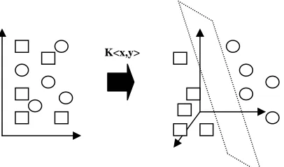
In Figure 1, the optimal hyperplane (solid line) is defined as the one the maximal margin of separation between the two classes. It can be uniquely constructed by solving a constrained quadratic optimization problem. The output from this solution is the support vectors (SV) (inside dot circle near dash line) that will be used for classification.
Figure 1: SVM classification example for separable two classes.
To increase the classification ability for non separating data, SVM map the data into a higher dimension feature space with kernel function K(x,y) where the data has much more possibility to be separated, then use a hyperplane in this feature space to separate the data as shown in Figure 2.
f(x)= -1
W,x + b = -1
Figure 2: SVM map data into higher dimension feature space in which the data have a much greater chance of being linearly separable.
SVM construct the maximum hyperplane by solve optimization problem defined by:
∑
∑ ∑
= = =
α α α − α
N
1 i i N
1 i
N
1
j i j i j i j
) x , x ( K y y 2
1
min (3)
With constraint:
∑
== α
N
1 i i i
0 y
N ,...., 1 i C
0≤αi ≤ =
Where
K (xi, xj) = Kernel function.
αi ,αj = Lagrange multipliers
yi ,yj = Training output sample
xi , xj = Training input sample
N = Number of training sample
C = Capacity control
The optimization processes will produce a Lagrange multipliers (α) and bias (b) values that will be used for classification. For predicting output (Ypredict) using new
data input(Xtest), equation below will be used :
b ) x , x ( K y
Y N
1 i
M
1
j train test train predict =
∑ ∑
α += = (4)
Where
K (xtest, xtrain) = Kernel function.
α = alpha value for SV
ytrain = Training output value
xtrain= Training input value
xtest = Testing input value
Ypredict = Predicted output value
N = Number of training sample
M = Data dimension
3.
KERNEL AND CAPACITY CONTROL(C)
SETTINGIn order to get a good performance of the SVM classifier, there are two points that must be considered carefully which are kernel function and capacity control (C). Kernel function K (xi, x) is used to map the
nonlinear input into a higher dimensional feature space, in which the learning capability of the machine is significantly increased. This kernel function will enable the operations to be performed in the input space rather than in the potentially high dimensional feature space. Hence, the inner product does not need to be calculated in the feature space. In this paper three common kernel functions which are Linear, Polynomial and Gaussian Radial Basis Function (GRBF) were tested. These kernel function capabilities were compared and the one that gives the higher accuracy in training and testing will be used in the real time system.
The detail algorithm for each kernel is shown below:
1. Linear Kernel
'
.
)
'
,
(
x
x
x
x
K
=
(5)2. Polynomial Kernel
d
x
x
x
x
K
(
,
'
)
=
(
.
'
+
1
)
(6)3. Gaussian Radial Basis Function Kernel
⎟
⎟
⎠
⎞
⎜
⎜
⎝
⎛
−
−
=
22
2
'
exp
)
'
,
(
d
x
x
x
x
K
(7)Choosing a suitable parameter for capacity control (C)
is crucial for good performance during training.
Generally, C controls between how hard to have a
large margin and how hard to avoid training error. As
C getting large, the solution with minimum training
error is acquired and increment in C beyond this point
will have no effect. This point cannot be overemphasized because training SVM with an
excessively large value of C tends to increase the
required training time by several orders of magnitude.
On the other hand, if C is too small, it will manifest
itself in a solution with no unbounded support vectors,
and therefore no ability to determine the bias (b) term
[10].
For simplification, the step for classification using SVM can be summarized as below:
1. Prepare the pattern of input-output matrix.
2. Choose the best kernel function.
3. Select the parameter of the kernel function
and the capacity control (C).
4. Execute the training algorithm using quadratic
programming optimization to obtain the values of α.
5. Classified unseen using α value and the
support vectors.
4.
RESULTFor real time mode application, the selected kernel function must attain a high performance in training and testing with a minimum number of support vector (SV). Figure 3 up to Figure 8 show the performance of training and testing with number of support vectors, for several kernel functions that based on training and testing data. The training data acquired from MIT database [11] consists of 386 images (212 of human images and 174 of vehicle images), while the testing data consists of 114 images taken from the video sequences of outdoor scene in [12]. The input feature consist of the selected best five HU moment values in [12] whereas the output classes is assigned to +1 for human and -1 for vehicle.
From simulations, value of C that is greater than
100 produced a static percentage performance (training and testing) and number of support vector (SV). Thus,
only a range of C that lies from 1 to 100 has been
analysed in detail. Also, only the polynomial function with a power of 2 and 3 is considered. As for Gaussian
Radial Basis Function (GRBF), apart from C the width
parameter (d) is also tested simultaneously. For this
reason, a cross intersection between these two
parameters (C and
d
∈
{
0
.
1
to
1
}
) consist of 1000combinations, equipped to the kernel function have been analyzed.
[image:4.612.318.538.109.234.2]Result for Linear Kernel Analysis
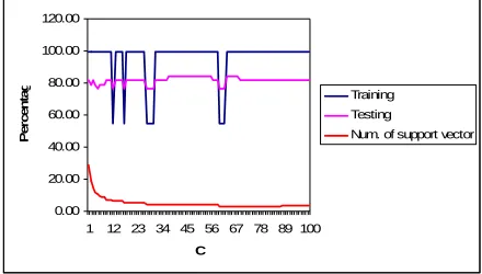
Figure 3 shows the result for linear kernel analysis. From the graph, linear kernel function shows
that with the increment of C, the performance for both
training and testing fluctuate between minimum of 54.92%(training) and 76.32%(testing) to maximum of 99.48%(training) and 84.21%(testing) , while the number of support vectors decreased constantly. From
the graph analysis, C = 63 gave the highest
performance of training (99.48 %) and testing
(84.21%) with lowest magnitude of support vector capacity (3.11%).
0.00 20.00 40.00 60.00 80.00 100.00 120.00
1 12 23 34 45 56 67 78 89 100
C
P
e
rcen
ta
g
Training
Testing
Num. of support vector
Figure 3. Percentage performance for testing, training and number of SV versus C for linear kernel.
Result for Polynomial Kernel Analysis
Figure 4 and 5 show the analysis result for polynomial power of two and three respectively. For polynomial kernel of power of two and three, the performance for
training achieved 100% as the C value reached above
74 (polynomial 2) and 34 (polynomial 3).The analyzed testing performance and capacity of support vectors
beyond these two C values gave 86.84% of testing
performance with 2.59% of support vectors for C=76
(polynomial 2), and 84.21% of testing performance
with 2.59% of support vectors for C=34 (polynomial
3).
0.00 20.00 40.00 60.00 80.00 100.00 120.00
1 12 23 34 45 56 67 78 89 100
C
Per
c
e
n
ta
g
Training Testing
Num. of support vector
[image:4.612.319.540.468.593.2]0.00 20.00 40.00 60.00 80.00 100.00 120.00
1 12 23 34 45 56 67 78 89 100
C
P
e
rcen
ta
g
Training
Testing
[image:5.612.318.542.72.206.2]Num. of support vector
Figure 5. Percentage performance for testing, training and number of SV versus C for polynomial power of 3.
Result for GRBF Kernel Analysis
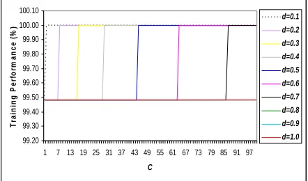
Figure 6, 7, and 8 show the analysis result for Gaussian Radial Basis Function (GRBF) for training, testing, and number of support vector (SV) respectively. GRBF shows that the highest performance in training and testing can be achieved when the combination of small
value of
α
and C were supplied, as α increased, thebigger C value need to be selected in order to give the
best performance. From Figures, it showed that d range
from 0.8 to 1 does not achieved 100% performance in training, so it has been discarded. For the rest of the width parameters (0.1 to 0.7), 100% performances in training and 86.84 performances in testing is achieved. The highest of SV capacity obtain by these parameters is 3.63% while the lowest one is 2.07%.
99.20 99.30 99.40 99.50 99.60 99.70 99.80 99.90 100.00 100.10
1 7 13 19 25 31 37 43 49 55 61 67 73 79 85 91 97
C
Tr
a
ini
ng P
e
rf
or
m
a
nc
e
(
%
)
d=0.1 d=0.2 d=0.3 d=0.4 d=0.5 d=0.6 d=0.7 d=0.8 d=0.9 d=1.0
Figure 6. Training performance versus C for GRBF width (d) of 0.1 to 1.
70.00 72.00 74.00 76.00 78.00 80.00 82.00 84.00 86.00 88.00
1 7 13 19 25 31 37 43 49 55 61 67 73 79 85 91 97
C
T
e
s
ti
n
g pe
rf
or
m
a
n
c
e
(
%
)
[image:5.612.74.293.73.198.2]d=0.1 d=0.2 d=0.3 d=0.4 d=0.5 d=0.6 d=0.7 d=0.8 d=0.9 d=1.0
Figure 7. Testing performance versus C for GRBF width of 0.1 to 1.
0.00 5.00 10.00 15.00 20.00 25.00 30.00 35.00
1 7 13 19 25 31 37 43 49 55 61 67 73 79 85 91 97
C
S
V
C
a
p
a
c
ity
(%
)
d=0.1 d=0.2 d=0.3 d=0.4 d=0.5 d=0.6 d=0.7 d=0.8 d=0.9 d=1.0
[image:5.612.318.542.257.390.2] [image:5.612.73.294.459.589.2]The results for the best cross intersection parameters
between C and d from Figure 3 to 8 can be summarized
[image:6.612.80.303.151.343.2]in Table 1 below.
Table 1. Performance for several kernel functions for classifies training and testing data.
Kernel d C Training
(%) Testing (%) Capacity SV (%) Linear
Poly. 2 Poly.
3 GRBF
- - - 0.1 0.2 0.3 0.4 0.5
0.6 0.7
0.8 0.9 1
63 76 34 3 8 17 33 46
67 91
85 50 62
99.48 100 100 100 100 100 100 100
100 100
99.48 99.48 99.48
84.21 86.84 84.21 86.84 86.84 86.84 86.84 86.84
86.84 86.84
84.21 84.21 84.21
3.11 2.59 2.59 3.63 3.63 2.59 3.11 2.59
2.07 2.07
3.11 3.11 3.11
From Table 1, it can be clearly seen that the entire selected kernel parameter excluding linear kernel and
GRBF with d larger than 0.8, gave a 100%
performance in training and 86.84% performance in testing. However, as for the support vector capacity,
GRBF with d=0.6 (C=67) and d=0.7 (C=91) gave the
lowest capacity (2.07%) though it posses the same
performances as others. However, since d=0.6 gave a
larger margin (0.147696) than d=0.7 (0.126733), thus,
it will be used in the real time mode.
5.
C
ONCLUSIONSIn this paper, a system to classify between human and vehicle using Support Vector Machine (SVM) classifier is discussed under dynamic pose. From the analyses, SVM training session via Gaussian Radial
Basis Function (GRBF) with C=67 and d=0.6 gave the
highest performance in training and testing, with only need eight of support vector (SV). The proposed SVM model gave a good result in 100% during training and 86.84% during testing.
In future, the system can be improve by extend the classification framework to other object classes like groups of people or sub classes like cars, vans, trucks, and motorcycles. A hierarchical multi class SVM probably best for this purpose by training the data using one versus all method.
R
EFERENCES1. Dengsheng Zhang, 2002. Image Retrieval Based
on Shape, Ph.D Thesis, Monash University.
2. Zhou Q and Aggarwal J. Tracking and Classifying
Moving Objects from Video. In Proc. 2nd IEEE
Int'l Workshop on Performance Evaluation of Tracking in Surveillance Dec 9 2001. Kauai, Hawaii.
3. Daniel Toth and Til Aach. Detection and
Recognition of Moving Objects Using Statistical
Motion Detection and Fourier Descriptors. 12th
International Conference on Image Analysis and Processing 2003. Washington, DC.
4. Burges, CJC. A tutorial on support vector
machines for pattern recognition. Data Mining
Knowledge Discovery 1998; 29(2):121–167.
5. Osuna E, Freund R, and Girosi F. Training
support vector machines:An application to face
detection. Proc. Computer Vision and Pattern
Recognition 1997; Puerto Rico:130–136.
6. Lou T, Kramer K, Goldgof D, Hall L, Sampson S,
Remsen A, Hopkins T. Learning to recognize
plankton. IEEE International Conference on
Systems, Man & Cybernetics October 2003; Washington, D.C: 888-893.
7. Zhang Qizhong and Zhejiang. Gene Selection and
Classification Based on Expression Data. In Proc.
IEEE/ICME International Conference on Compex Medical Engineering (CME 2007) May 23-27 2007. Beijing
8. Liang Zhao and Takagi N. An Application of
Support Vector Machine to Chinese Character
Classification Problem. In Proc. Of IEEE
International Conference on System, Man and Cybernatics (ISIS 2007) October 7-10 2007. Montreal.
9. Dumais, ST, Platt J, Heckerman D, and Sahami
M. Inductive learning algorithms and
representations for text categorization. Proc.
ACM-Conf. Information and Knowledge Management (CIKM98) Nov 1998. Bethesda, Maryland; 148–155.53
10. Rifkin, RM.,2002. Everything Old is New Again:
A Fresh Look at Historical Approaches in Machine Learning, Ph.D Thesis, Massachusetts Institute of Technology, Boston USA.
11. http://cbcl.mit.edu/software-datasets/
12. Razali M.T and Adznan B.J. Detection and
Classification of Moving Objects for Smart Vision
Sensor. In Proc. of 2nd IEEE International