The effect of pile weight to the capacity of pile

THE EFFECT OF PILE WEIGHT TO THE CAPACITY OF

PILE

AGUS SULAEMAN

MALEK ABDUL RAHMAN

PROSIDING KEBANGSAAN AWAM '07,

LANGKAWI, KEDAH (AWAM 2007)

A w / ' A W A M 2 0 0 7

The Effect of Pile Weight to the Capacity of Pile

'Agus Sulaeman, 2M a l e k bin Abdul Rahman

1 2

Lecturer, Researcher, Faculty of Civil & Environmental Engineering, Universiti Teknologi Tun Hussein Onn, Parit Raja, Batu Pahat, Johore.

Abstract

It has been recognized that the pile capacity depends upon pile size and soil condition, the effect of pile weight has never been considered. In order to unveil this matter, the small scale modeling technique (1 g) is one of the proper ways to solve due to the fact that full scale pile loading test cannot accommodate this case. Small Scale model frame apparatus furnished with high accuracy instrumentations has been set up at Kuittho, a series of different pile weight models, several tests and analysis of model to prototype similarity has been conducted. The conclusion reveals that the lighter pile exhibit additional significant capacity compare to the pile made from normal concrete weight, from this reasons, a lighter concrete pile as an alternative pile material can be developed to obtain the lightest pile as long as it complies with strength and stability requirements.

Keywords: Lightweight concrete, capacity, similarity, physical model, pile weight

1.0 Introduction

Foundation design can only be advanced by theories that are related to observed foundation behavior. Even designs using well established theories may require repeated reference to field tests. However, testing a full scale foundation structure is costly, time consuming and often impossible. For these reasons, testing is normally limited to the observations of the behavior of small models that duplicate the actual structure (the prototype) in some proportion.

Under condition of normal gravity, model tests are easy to perform. However, when applying the results of a small scale model test to predict the behavior of a prototype structure, simply scaling the test result to the ratio of geometric size is not sufficient.

The prediction must also consider the stress levels acting in the soil of the model test in reference to those at homologous points in the soil of the prototype structure. If this is neglected, the applicability of the

tests results to the intended foundation problems can be substantially disrupted.

To overcome the problem associated with 1 g physical model tests, there are 2 solutions which based on similarity principle:

1. The tests can be made in the centrifuge where centrifugal acceleration replaces the gravity so that the stress at all homologous points of the model is equal to the stress induced by gravity in the actual foundation.

2. Employing critical state line concept. This scrutinized work has been done by Fellenius to the sandy soil to obtain the similarity.

This paper presents an application of critical state line concept applied to clay soil to find out the effect of pile weight to its capacity.

1.1 Similarity relationship

A series of similitude theory from the beginning Buckingham n theory (1910) to

A W A M 2007

Prosiding Kebangsaan Awam '07, Langkawi, Kedah, 29hb - 31hb Mei 2007

n = Lm / LD (1)

where Lm is the length dimension in the

model and Lp is the length dimension in the

prototype

2. The stress scale ratio N

N = a\ ₍₂₎

where a< = effective stress in the model at

m

homologous point, a' = effective stress in

the prototype at homologous point

Use of small scale models require a scaling relation between stress and strain that builds on an understanding of how void ratio ( density ) of the soil changes following a change of stress, this concept has been explained by Cassagrande ( 1936 ) on the term critical void ratio.

Then Roscoe et al. ( 1963 ) developed the Cassagrande concept into defining a state at which the soil continue to deform at constant stress and constant void ratio.

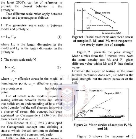
Utilizing this concept, More recently Fellenius (1994 ) described the result of 3 CD test on crushed quartz sand , the samples P, Mi and M 2 were tested at different initial void ratios and initial mean stresses as cited in the Figure 1. Other results are shown in the figures below.

Void _atio

state line

Ln mean stress (kPa)

F i g u r e l : Initial void ratio and mean stress of samples P, Mi and M 2 with respect to

the steady state line of sample.

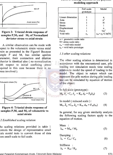
Figure 2 presents the peak strength Mohr circles from the 3 triaxial tests, Note the same density test M 2 and P gives different value whilst Mi and P has similar value.

However the aspect of testing at the same lambda parameter does not just address the peak strength, but the entire behavior of the soil.

Shear stress Tangent to M2

Tangent to M l & P

/ M 2 , - , * Ml \ P

\

\

Normal effective stress (kPa)

i 2 L

Figure 2: Mohr circles of samples P, Mi and M 2

Figure 3 shows the response of 3 samples, the curves representing samples P and Mi have the same upsilon parameter and, therefore their normalized behaviors are practically identical. Sample M 2 on the other hand exhibits a higher normalized stress strain curve because of its larger initial lambda parameter.

Pusat Pengajian Kejuruteraan Awam, Universiti Sains Malaysia

the latest 2000's can be of reference to provide the closest behavior to the prototype.

Two different scale ratios apply between a model and a prototype as follows:

/ A W A M 2 0 0 7

Prosiding Kebangsaan Awam '07, Langkawi, Kedah, 29** - 31hb Mei 2007

Figure 3: Triaxial drain response of samples P,Mi and M 2 of Normalized

deviator stress vs axial strain

A similar observation can be made with respect to the volumetric strain versus axial strain as presented in the Figure4 Because sample P and Mi has similar upsilon parameter, their contraction and dilation behavior is identical also ( no normalization with respect to initial confining stress required in this case because there is no stress involved).

Figure 4: Triaxial drain response of samples P,Mi and M 2 of volumetric vs

axial strain

1.2 Established scaling relation

The scaling relations provided in table 1 controls the design of representative small scale model tests to convert those of data from small scale to full scale.

Table 1: Scaling relations of the physical modeling approach

Full scale prototype

Model

Linear dimension Area

Stress Strain Displacement Force Void ratio

n n2

N 1 n N n2

em= ep+X ln(N)

n = geometric scale ratio N = stress scale ratio em - void ratio model

ep = void ratio prototype

1.3 other scaling relations

The other scaling relation is determined in accordance with the encountered case, pile loading test simulation needs time scaling relation to model the speed of loading in the model. The object in nature which can represent the pile motion during pile loading test can be simulated by equation of motion of the object:

In full scale (prototype) :

M p ^ + C p ^ + K p ^ F p O p ) (3)

In model ( reduced scale ) :

Mm Am + Cm AM +KmAm = Fm( tm) (4)

In general, for any given similarity analysis the following scaling factors apply to the equation of motion.

Mass : Xm = Mm/ Mp

Damping : Xc Cm / Cp

Stiffness :

(5)

>

Prosiding Kebangsaan Awam '07, Langkawi, Kedah, 29^b - 31hb Mei 2007

Velocity :

Xv= Vm/ Vp (10)

Acceleration :

Aa^Arn/Ap (11)

Time :

At = tm/ tp (12)

Substitution (6) to (13) into ( 5 ) :

Mm = A.m Mp ; Cm = XcCp ; Km = XK Kp;

Fm = X* Fp ; Lm = XL Lp ; V m = Xy Vp ;

A m = Xa Ap tm = Xt tp into (2)

{ XkXL/ XF} = l (18)

If model testing is done by a 1 - g environment, the scaling factor for acceleration = 1

Xa = A m / A p = 1 ; Xa = XL / Xt2 = 1 ; Xt2 = XL

X, = ( XL)0 5 (19)

hence tm/ tp= ( Lm / Lp ) 0 5

it means the scaling relation for time is

tm = tp( Lm/ Lp)0? (20)

{ XmXa} M p ^ + { XcXv} C p i/, +

{XkXL}KpAp = {XF}FP (tp ) (13)

However : Xy = XL / Xt ; Xg = XL / Xt2 ;

Xm ~ Xp . XVoi = Xp .XL

Provided that we enforce the condition \p = 1 density of the model similar to that of prototype w e can express

Xm = 1. XL3 or Xm = XL3 , Then in equation

(14)

{ Xv oi3XL/ Xt 2} M p ^ +

{Xc XL/Xt}Cp Ap+{XkXL}KpAp=

{ ^ } F p ( tp) (14)

Dividing m t m by { XF } :

{ XL 4/ Xt 2. l / XF} M p ^ +

{XkXL/XF}KpAp = F p ( tp) (15)

2.0 Scope of Investigation

The present research has been made to study the correctness of the similarity concept to cohesive soil to find out the effect of pile capacity based on different pile weight.

3.0 Test Procedure

The procedures of performing this physical modeling consist of some main works:

3.1 Preparation of small scale modeling equipment.

3.2 Obtaining similarity requirements 1. Triaxial CU tests to obtain critical

state line of clay soil sample X 2. Obtaining other parameters : Su and

ep

3. Set a geometry scale factor ( n ) 4. To obtain stress factor N refers to

Pusat Pengajian Kejuruteraan Awam, Universiti Sains Malaysia

For similarity to be fulfilled then the Force : following conditions should be satisfied :

h

{ AjjVXt2. 1/XF} = 1 (16)

Displacement:

/ A W A M 2 0 0 7

Prosiding Kebangsaan Awam '07, Langkawi, Kedah, 29hb - 3lhb Mei 2007

em= ep+X ln(N) or Figure 1, em value and

N can be adjusted. Soil condition at the model should have a value of em.

3.3 Conducting model tests

1. Preparing model soil with em

condition, various model pile in accordance with the planning.

2. Driving the model piles of different pile weight.

3. Loading test to various model piles at prescribed rate of load.

3.4 Conversion data from original small scale into full scale

3.5 Controlled their ultimate capacity by Numerical modelling.

4.0 Materials

4.1 Scaled loading test equipment

The test conducted in a scaled loading test which transparent glass at each side supported by steel frame and necessary appurtenance. The displacement transducer connected to data logger and digital loading display available to read data from loading cell, all this instrumentations are equipped with high sensitive measurements.

The box size is 1.2 m x 2.4 m x 1.2 m as shown in the figure 4. It was furnished with water tank to provide water with maintained water level. Loading frame and ram were installed to give the loading at certain rate.

Figure 5: Various model piles

4.2 Soil model

Soft clay soil sample was taken from Recess site inside Kuittho area by using common drilling equipment to a certain depth as needed, whereas soft clay for model soil was taken from similar location at similar depth. Soft clay model soil mixed with certain amount of water to form slurry to obtain em = ep + A, In N .

4.3 Pile model

Concrete model pile shown in the Figure5 consist of various length / diameter of 30 mm in diameter.

5.0 Testing On Small Scale Basis

The testing was undertaken in accordance with scaled geometry, stress and velocity prescribed earlier.

A W A M 2007

Prosiding Kebangsaan Awam '07, Langkawi, Kedah, 29hb - 31hh Mei 2007

Figure 6: Testing was being undertaken

Figure6 shows the tests was undertaking to measure displacement at prescribed loading in pile movement at certain rate.

Void Ratio v s Mean S t r e s s p' fkPal

100 0 0 0

Mean S t r t s s p' kPa

Figure 8: The result of Initial void ratio and mean stress of samples Prototype and model with respect to the steady state line

of sample.

To obtain soil model prescribed by em = ep

+ X In N , since the steady state line, XI =-0.003, X2=-0.003 , ep= 0.818 so em = 1.580

then N = 80/10 = 8

Figure 7: Data result stored in data logger

The data from load cell was recorded at panel provided and displacement recorded in data logger as shown in the Figure7.

6.0 Test Results And Analysis

6.1 Critical State line

The CSL of both lines which is parallel to one another can reflect the similarity it can be seen in the Figure 8. In a broader sense, the concept behind the steady state or critical void ratio satisfies the conditions for use as reference state for physical modeling.

6.2 The Comparison of Strength properties

The CU triaxial result of strength properties of model soil and the result of prototype along with strength envelope comparison is shown in the Figure 9 and Figure 10 respectively

Figure 9: Mohr Coulomb of model soil

To make sure that the similar behavior occur between them comparison was made by plotting strength envelope of model into prototype as shown in the figure 10. It can reveal that both line almost close each other, from this we can draw the conclusion that both soil exhibit almost similar behavior.

/ A W A M 2 0 0 7

Prosiding Kebangsaan Awam '07, Langkawi, Kedah, 29hh - 31hb Mei 2007

FigurelO: Plotted into prototype

In order to enhance this confidence, the supporting data from both triaxial test can be analyzed

Table 2: The strength properties result of model and prototype

M o d e l Prototype

Angle Sh resistance, _{10.22 8.35}

Cohesion, c (kPa) 3.69 7.01

Bulk Density, y ( k N / m3) 15.83 16.00

The strength properties result of both model and original as tabulated in the table 2 indicating the close value of angle of shear and cohesion.

6.3 The comparison of Shear stress vs axial strain

A similar observation can be made with respect to shear stress vs axial strain.

Comparing those of normalized shear stress vs axial strain of P and M reveals that similarity occur when both P and M was confined under similar cell pressure, it can be found in M2,M3 and P2,P3 as shown in the Figure 11.

The CU triaxial test can not measure the volume change, the pore water pressure can be provided instead, however no clear correlation of their behavior occurs. According to Fellenius in CD triaxial test, the close correlation is clear

T h e comparison of model and prototype

-5 0 5 10 15 20 25 30 axial strain

F i g u r e l l : Comparing normalized shear stress vs. axial strain of model and

prototype

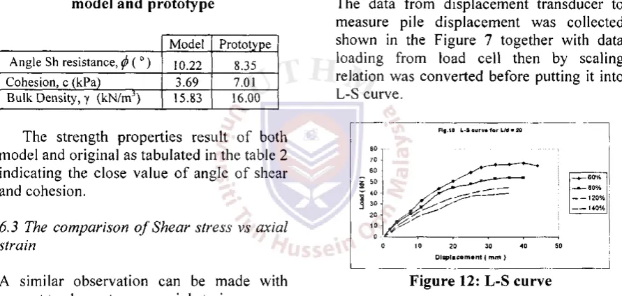
6.4 L-S curve

The data from displacement transducer to measure pile displacement was collected shown in the Figure 7 together with data loading from load cell then by scaling relation was converted before putting it into L-S curve.

Fig.10 L - S o u r v « f o r L / d « 2 0

Figure 12: L-S curve

From the pile load test conducted using the Slow maintain Load Test, the pile capacity is determined from the load-settlement curve measured through a plotted graph. The scaling relation in Table 1 was used to convert the force and displacement data gathered to establish this load-settlement curve.

/ A W A M 2 0 0 7

PresidingKebangsaanAwam'07, Langkawi, Kedah, 29hh

-Model Scaling

Relation

Prototype

L = 600 m m N = 8 ( L = 6 m

Dia. = 30 measured and Dia. = 300

m m calculated ) mm

em= 1.580 n=10 ep = 0.818

c= 3.69 kPa prescribed ) c = 7 . 0 1 k P a

</>= 10.22 ^ = 8.35

y= 15.83 y= 16.00

k N / m3 k N / m3

a). Using common available formula

Qu = QP + Qf

Qp = 9 C A p = 9 x 7.01 x JI/4 x 0 . 32

= 4.45 kN

Qf = Qf c + Qf>

Qf c= (15 x 0.3) 7.01/2 x 7i x 0.3 +

( 1.5 x 7.01 ) TCXO.3 = 14.83 + 9.89 = 24.72 kN

Qty = ( K Gv tan5 ) 7t 0.3 x 6 = 20.30 kN

Qu = QP + Qf

= 4.45 + 24.72 + 20.30 = 49.47 kN

b) Using converted L- S curve

The Qu resulted from L-S curve of converted data using common ultimate capacity interpretation method = 50 kN as shown in the Figure 12.

Those above results give an almost similar value, this is a proof of how importance the scaling relations are -neglecting this will be misleading.

31hh Mei 2007

F i g u r e l 3 : Numerical analysis by F E M

6.7 Curves for various L/d and weight

The data results which have been converted into full scale basic was then collected in table 4, and plotted in the curve as shown in the Figure 14

Table 4: The capacity of various pile

No. L/d No.

L/d

60 % 80 % 100 % 120 % 140 %

1 10 39 34 23 18

2 15 45 41 30 26

3 20 62 53 43 38

It reveals that the lighter the pile weight the bigger capacity they get compared to the reduction of weight from their weight alone, it can be seen clearly in the curves even though the increased capacity is slightly bigger.

6.6 Numerical analysis

The Calculation of bearing capacity can be made in F E M using available commercial software, this calculation was done to ascertain our analysis goes well.

Numerical analysis was made using triangular 15 node FE, axysimmetri, Mohr-coulomb soil model. The results from FEM as shown in the Figure 13 shows a good agreement to the results by common manual formula and physical model

The Figure 12 shows the load-settlement curve which has been converted to full scale condition.

6.5 Ultimate capacity by common formula

The analysis of small scale modeling should be compared to the ordinary result of common formula; the table 3 indicates the data to be used for calculation.

A W A M 2007

Prosiding Kebangsaan Awam '07, Langkawi, Kedah, 29hh - 31hb Mei 2007

Fig.13 Ultimate capacity c o m p a r e to ult. Cap.of n

70

•t5 0

*

I 20 = 10

- U d = 20

Ud = 15 - U d = 10

- normal concrete - normal concrete -normal concrete

50 100 150 Percentage to normal concrete %

F i g u r e l 4 : The ultimate capacity of various weight compare to normal weight

concrete

7.0 Conclusion

1. The similarity requirements is needed in performing analysis and design in small scale physical modeling either applied in sand or clay soil.

2. The more lighter the bigger capacity of pile.

Acknowledgements

The authors would like to express their grateful for the financial support from the PPB KUiTTHO (former name of UTHM ) and Research Centres ( RECESS) KUiTTHO for providing scaled loading test and other supporting equipments.

Reference

Atkinson, J.H., and Bransby, P.L., 1978, THE M E C H A N I C S OF SOILS, An Introduction to critical state soil mechanics., Mc Graw Hill

Fellenius,B.H.1994 Physical modeling in sand, Canadian Geotechnical Journal,Ottawa, pp.420-4313. Neville,A.M. and Brooks,J.J.( 1993). Concrete Technology. Longman

Noor, F.A. and Boswell . (1991) SMALL SCALE PHYSICAL MODELLING, Elsevier Applied Science, London and NewYork

Prakash, S and Sharma, H.D. , 1990, PILE F O U N D A T I O N IN ENGINEERING PRACTICE, John Wiley and Sons, New York

Roscoe, K.H., and Poorooshasb, H.1963. A fundamental principle of similarity in model test for earth pressure problems. In proceedings of the 2n d Asian Regional

Conference on Soil Mechanics, Bangkok, Thailand. Vol l . p p . 1 3 4 - 1 4 0

Schofield, A.N., and Wroth, C P . 1968. Critical state soil Mechanics, McGraw-Hill, London.

Scott, R. F. 1988. Physical and Numerical models In Centrifuge in soil mechanics, Edited by W.H. Craig, R.G. James. AA Balkema, Rotterdam. Pp. 103-117