Representing Data Distributions with a Nonparametric Kernel Density: The Way to Estimate the Optimal Oil Contents of Palm Mesocarp at Various Periods

Representing Data Distributions with a Nonparametric

Kernel Density: The Way to Estimate the Optimal Oil

Contents of Palm Mesocarp at Various Periods

Divo Dharma Silalahi

1,2,*

_{, Putri Aulia Wahyuningsih}

1

_{, Fahri Arief Siregar}

1

1_{SMART Research Institute, PT SMART Tbk, Indonesia} 2_{Institute of Statistics, University of the Philippines Los Baños, Philippines}

*Corresponding Author: [email protected]

Copyright © 2013 Horizon Research Publishing All rights reserved.

Abstract

The most popular nonparametric density estimates is kernel density estimate. This estimate depends on the bandwidth choice which was given the optimization to kernel optimality process. We proposed Epanechnikov kernel which is the most optimal kernel in the AMISE. The resample data as replicate samples has been obtained by using bootstrap mechanism to provide the information about the sampling distribution. Then the resample data was used in Epanechnikov kernel simulation to estimate the optimal solution. This study was simulated using oil contents (%) data at various periods after pollination. The oil contents (%) were obtained by extraction of oil palm mesocarp. The result show that, Epanechnikov kernel using resamples data from bootstrap could be used for nonparametric optimization cases such as oil content (%) of oil palm mesocarp.

Keywords

Nonparametric, Epanechnikov Kernel, Density Estimation, Bootstrap, Optimization, Oil Palm Mesocarp

1. Introduction

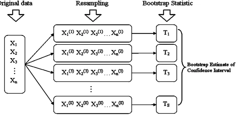
Bootstrap mechanism was introduced in 1979 as a computational statistical technique that allows making some inferences from data without making strong distributional assumptions [1]. As problem with small sample size, bootstrap mechanism can be used to resample the set of data with replacement to estimate the statistic’s sampling distribution. The sampling distribution if it can be

[image:1.595.313.553.477.651.2]

determined may then be used to estimate standard errors and confidence intervals for that particular statistic. Although the data point has been used, it is not deleted from the original data set or, using the usual terminology, which is replaced. As a result, the same observation may be included in the resample data set. In this case, we used the bootstrap mechanism to resample oil contents of palm mesocarp data at 10 periods (week: 6, 14, 16, 18, 19, 20, 21, 22, 24, 26) after pollinations. This field study was conducted in South Kalimantan, Indonesia. The data was obtained from laboratory analysis as extracted process to fresh fruit oil palm samples with variety is progeny-66 and genotype-03. We only have 3 replicates per period, and then we generated the data using bootstrap become 250 replicates.

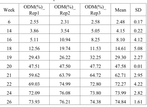
Table 1. Descriptive statistic oil contents of %ODM Week ODM(%)_ _Rep1 ODM(%)_ _Rep2 ODM(%)_ _Rep3 Mean SD

6 2.55 2.31 2.58 2.48 0.17

14 3.86 3.54 5.05 4.15 0.22

16 5.11 10.94 8.25 8.10 4.12

18 12.56 19.74 11.53 14.61 5.08

19 29.43 26.22 32.25 29.30 2.27

20 47.51 47.50 47.72 47.58 0.01

21 59.62 63.79 64.72 62.71 2.95

22 69.03 74.99 72.80 72.27 4.22

24 72.09 76.08 73.80 73.99 2.82

26 73.93 76.21 74.38 74.84 1.61

[image:2.595.113.504.84.358.2]

Figure 1. Oil contents of palm mesocarp in 3 replicates

A very natural use of density estimates is in the informal investigation of the properties set of resamples data. Density estimates can give valuable indication of such features as skewness and multimodality in the data. In some cases they will give conclusion that may then be regarded as self-evidently true further to data collection. This density referred to Epanechnikov kernel density estimates that used in simulation to estimate the optimal oil contents of palm mesocarp at those periods. The analysis was processed using auxiliary software such that: R version 2.15.2 and Stata 12.

2. Bootstrap

2.1. Definition

The Bootstrap is a resample mechanism designed to provide information about the sampling distribution of a functional

T

(X

₁

,

X

₂

,



,

X

_n

,

F)

where

X

₁

,

X

₂

,



,

X

_n

are sample observations and

F

is CDF from which

n 2

1

,

X

,

,

X

X



are independent observations. The

bootstrap is not limited to the iid situations. It has been studied for various kinds of dependent data and complex situations. In fact, this versatile nature of the bootstrap is the principal reason for its popularity. There are numerous texts and reviews of bootstrap theory and methodology, at varied technical level [1] [2].

Suppose

X

1

,

X

2

,



,

X

niid

~

F

and

T

(X

1

,

X

2

,



,

X

n

,

F)

is a functional, e.g.,

σ

μ)

X

(

n

F)

,

X

,

,

X

,

(X

T

_{1 2}

_

_n

=

−

,

where

μ

=

E

_F

(X

₁

)

and

σ

2

=

Var

_F

(X

₁

)

.

In statistical problems, we frequently need to know something about the sampling distribution of

T

,

e.g.,

t)

F)

,

X

,

,

X

,

(T(X

P

F 1 2



n

≤

.

If we have replicated samples from the population, resulting in a series of values for the statistic

T

, then we could form estimates of

P

_F

(T

≤

t)

by counting how many of the

T

_i’s are

≤

t

. But statistical sampling is not done using that way. Replicate samples were not usually obtained, but otherwise only one set of data of some size

n

[1].

A large sample from a finite population should be well representative of the full population itself. Suppose for some number

S

, we draw

S

resample of size

n

from the original sample. The resample were denoted from the original sample as

),

X

,

,

X

,

(X

*11 *12



*1n

(X

*21

,

X

*22

,



,

X

*2n

),

…,

),

X

,

,

X

,

(X

*S1 *S2



*Sn

with corresponding values

T

₁*

,

T

₂*

,



,

T

_S* for the functional

T

, we can use simple frequency based estimates

such as

{

}

B

T

:

j

#

*

2. Bootstrap Distribution and

Consistency

The formal definition of the bootstrap distribution is the following

Let

X

1

,

X

2

,



,

X

niid

~

F

and

T

(X

1

,

X

2

,



,

X

n

,

F)

is

a given functional, the ordinary bootstrap distribution of T is defined as

x)

F)

,

X

,

,

X

,

(T(X

P

)

(

H

Boot

x

=

Fn 1 2



n

≤

where

(X

*₁

,



,

X

*_n

)

is an iid sample of size

n

from the empirical CDF

F

n .

P

* is common used to denote

probabilities under the bootstrap distribution [4].

At first glance, the idea appears to be a bit too simple to actually work. But one has to have a definition for what one means the by the bootstrap working in a given situation. For estimating the CDF of a statistic, one should want

(x)

H

Boot to be numerically close to the true CDF

H

n

(x)

of

T

. For a general metric

ρ

the definition is the following Let

F

,

G

be two CDFs on a sample space

X

. Letρ(F,G) be a metric on the space of CDFs on

X

. For

X

₁

,

X

₂

,



,

X

_niid

~

F

, and

a

given functional

F)

,

X

,

,

X

,

(X

T

1 2



n , let

   



 _≤

   

 

=P X ,X , ,X ~F x (x)

Hn F 1 2  niid (1)

   



 _≤

  

 

=P X ,X , ,X ~F x (x)

HBoot * 1* 2*  n*iid (2)

The bootstrap is weakly consistent under

ρ

for

T

if

(

H

,

H

)

0

ρ

n Boot

⇒

P as

n

→

∞

. Otherwise, bootstrap is

strongly consistent under

ρ

for

T

if

ρ

(

H

n

,

H

Boot

)

⇒

as..

0

[4].

2.3. Bootstrap Confidence Interval

In a series of article, Efron [5] [6] [7] [8] [9] has introduced and refined the percentile method. This was using bootstrap calculations to set approximate confidence interval for scalar parameters. These refinements of the percentile method are the bias-corrected (BC) percentile method and the accelerated bias-corrected (BCa) percentile method. Efron’s approach is to first develop these procedures in the simple context of a parametric model indexed by a scalar parameter, for which there are no nuisance parameters present, and then to adapt them for application in multiparameter families and nonparametric situations.

For a review of the percentile method in the simplest case, suppose that Let

G

ˆ

be the cumulative distribution of

θ

ˆ

*. The 1−2

α

percentile interval is defined by the

α

and

α

−

1

percentiles of

G

ˆ

:

(

θ

,

θ

)

(

G

1

(

)

G

1

(1

α)

)

up %, lo

%,

ˆ

=

ˆ

−

α

,

ˆ

−

−

ˆ

₍₃₎

Since by the definition

(

*( ) *(1α)

)

-1

₍

_α

_θ

_,

_θ

G

ˆ

₎

₌

ˆ

α

ˆ

−

the100⋅αth percentile of the bootstrap distribution, we can also write the percentile interval as

(

) (

*(α) *(1α)

)

up %, lo

%,

,

θ

θ

,

θ

θ

ˆ

ˆ

₌

ˆ

ˆ

− ₍₄₎

[image:3.595.117.502.539.730.2]

These are the ideal bootstrap situation in which the number of bootstrap replications is infinite. In practice we must use some finite number of replications. Then the arguments in favor of the percentile interval should translate into better coverage performance.

3. Kernel

3.1. Kernel Density Estimation

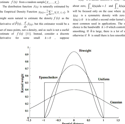
We limit the kernel overview only to the nonparametric case as this is the one primarily used in computer graphics, in other side the illumination of a scene seldom can be described adequately by a simple function. A general nonparametric density estimator is the kernel estimator. The kernel estimator approximates a density function by weighting the samples of a dataset by their distance to the position. This is done using a kernel function.

Let X is a random variable with continuous distribution

F(x)

and density _F(x)

dx d (x)

f = . The objective is to

estimate

f

(x)

from a random sample

{

X₁,,X_n

}

. The distribution function F(x) is naturally estimated by

the Empirical Density Function

₍

₎

1 1

F(x) 1

n

n i i= X x

=

∑

≤ . It

might seem natural to estimate the density

f

(x)

as the derivative of

F

ˆ

(x)

, _F(x)

dx

d _{ˆ , but this estimator would be a}

set of mass points, not a density, and as such is not a useful estimate of

f

(x)

[11]. Instead, consider a discrete derivative for some small h>0 , suppose

2h h) -(x F -h) (x F (x)

fˆ = ˆ + ˆ ; we can write this as

(

)

n n

i i

i 1 i 1

X x 1 _{1 x h X x h} 1 _{1 1} 2nh = 2nh = h

 −  + < ≤ + = _ ≤ _

 

∑

∑

n i

i 1

X x

1

_k

nh

=

h



− 









∑

n i

i 1

X x

1

ˆf (x)

k

nh

=

h

−





=

_

_





∑

(4)

where

k(u)

is a kernel function.

k(u)

is a kernel function if

k(u)

=

k(-u)

symmetric about zero,

∫

∞

∞

−

k(u)du

=

1

and

∫

∞

∞

−

k(u)du

=

0

.

This

will be focused only on the case where k(u)≥0 so that k(u) is a symmetric density with zero mean. When

0

k(u)

≥

it is called a second order kernel and these is the most common used in applications. The most important choice is the bandwidth

h

>

0

which controls the amount of smoothing. If

h

is large, there is a lot of smoothing, and otherwise if

h

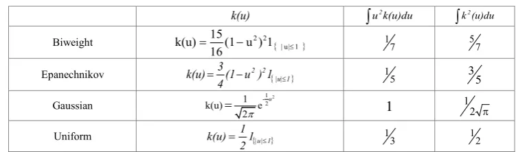
is small there is less smoothing [11].

[image:4.595.58.493.257.685.2]

[image:5.595.114.490.88.199.2]

Table 2. Several types of kernel density estimation

k(u)

_∫

u2k(u)du

∫

k2(u)du

Biweight k(u)=15₁₆(1−u2)21{|u|≤1} 1₇ 5₇

Epanechnikov k(u)=3₄(1−u2)21_{|u|≤1_} 1₅ 3 5

Gaussian _k(u) 1 _e-122

2

u π

= ₁ 1_{2 π}

Uniform k(u)=1₂1{|u|≤1} 13 12

Based on some literature for kernel smoothing and optimization [10], performance of kernel is measured by Mean Integrated Squared Error (MISE) or Asymptotic MISE (AMISE). Epanechnikov kernel is the optimal kernel in the AMISE. Which is kernel efficiency is measured in comparison to Epanechnikov kernel. Based on this literature we used Epanechnikov kernel as a weighting function with

otherwise 1 | u | 0 ), u -(1 4 3

k(u) 2 ≤

   

= (5)

3.2. Density Estimator

First if

k(u)

is non-negative then it is easy to see that

0

(x)

f

ˆ

≥

. However, this is not guaranteed if k is a higher order kernel. In this case it is possible that fˆ(x)<0 for some values of

x

. When this happens it is prudent to zero out the negative bits and then rescale [11]:

∫

∞∞

≥

≥

=

-

f

(x)1(

f

(x)

0)dx

0)

(x)

f

(x)1(

f

(x)

f

ˆ

ˆ

ˆ

ˆ

ˆ

(6)

(x)

f

ˆ

is non-negative yet has the same asymptotic properties as

f

ˆ

(x)

. Since the integral in the denominator is not analytically available this needs to be calculated numerically.

( )

u

du

1

k

dx

h

x

X

k

h

1

i

_

₌

₌











−

∫

∫

−∞∞ ∞ ∞ − Thus n i i 1 n i i 1 1

X x

1

1

ˆf(x)dx

k

dx

n

h

h

X x

1

_{1 k}

_dx

n

h

h

1 1 1

n i

n

∞ ∞ −∞ −∞ ∞ −∞ = = =

−





=

_

_





−





=

_

_





=

=

∑

∫

∫

∑∫

∑

As claimed. Thus

f

ˆ

(x)

is a valid density function when

k

is non-negative [12].

We can also calculate the numerical moments of the densityfˆ(x). By using the change of variable

(

)

h x X u₌ i− _,

the mean of the estimated density is n i i 1 n i i 1

X x

1

1

ˆ

xf(x)dx

x k

dx

n

h

h

X uh

1

_k(u)du

n

h

∞ ∞ −∞ −∞ ∞ −∞ = =

−





=

_

_





+





=

_

_





∑

∫

∫

∑ ∫

(7) n n i

i 1 i 1

n i i 1

1 _{X k(u)du} 1 _{h u k(u)du}

n n 1 _X n ∞ ∞ −∞ −∞ = = = = + =

∑

∫

∑

∫

∑

(7)

The second moment of the estimated density is

(

)

n

2 2 i

i 1 n ₂ i i 1

X x

1

1

ˆ

x f(x)dx

x

k

dx

n

h

h

1

_{X uh k(u)du}

n

∞ ∞ −∞ −∞ ∞ −∞ = =

−





=

_

_





=

+

∑

∫

∫

∑ ∫

n n 2 i i

i 1 i 1

n 2 2 i 1 n 2 2 i 2 i 1

1

_X

2

_{X h}

_k(u)du

n

n

1

h

u k(u)du

n

1

_X

_{h k (k)}

n

∞ −∞ ∞ −∞ = = = =

=

+

+

=

+

∑

∑ ∫

∑ ∫

∑

(8)

It follows that the variance of the density

f

ˆ

(x)

is

(

)

2

2

2

n n

2 2 2 2

i 2 i 2

i 1 i 1

ˆ

ˆ

x f(x)dx -

x f(x)dx

1

_X

_{h k}

1

_X

_σ

_{h k (k)}

n

n

∞ ∞ −∞ −∞ = =

=





=

+

−

_

_

=

+





∫

∫

∑

∑

(9) 2

σˆ is the sample variance. Thus the density estimate inflates the sample variance by the factor

h

2

k

₂

(k)

.

It is useful to observe that expectations of kernel transformations, which can be written as integrals that take the form of a convolution of the kernel and the density function [12] [13] [14]:

f(z)dz

h

x

z

k

h

1

h

x

X

k

h

1

E

i

_









 −

=













−

∫

−∞∞

Using the change of variables

u

=

(

z

−

x

)

/

h

this equals to

( )

u

f(x

hu)du

k

+

∫

−∞∞

By the linearity of the estimator we can see n i i 1

X x

1

1

ˆ

E f(x)

E k

n

h

h

_−∞∞

k(u)f(x h u)du

=

−





=

_

_





=

+

∑

∫

(10)

This integral (typically) is not analytically solvable, so we approximate it using Taylor expansion [13] [14] of

hu)

f(x

+

in the argument hu, which is valid as hu→0. For a

v

’th order kernel we take the expansion out to the

v

’th term

)

o(h

u

(x)h

f

v!

1

u

(x)h

f

3!

1

u

(x)h

f

2

1

(x)hu

f

f(x)

hu)

f(x

v v v (v) 3 3 (3) 2 2 (2) (1)

+

+

+

+

+

+

=

+



The remainder is of smaller order than

h

vas

h

→

∞

, which is written as

o(h

v

)

. Integrating term by term and using

∫

∞ k

( )

u du=1

∞

− and definition k

( )

uu du kj(k)

j ₌

∫

−∞∞

( )

)

o(h

(k)

k

(x)h

f

v!

1

f(x)

)

o(h

(k)

k

(x)h

f

v!

1

(k)

k

(x)h

f

3!

1

(k)

k

(x)h

f

2

1

(k)

(x)hk

f

f(x)

hu)du

f(x

u

k

v v v (v) v v v (v) 3 3 (3) 2 2 (2) 1 (1)

+

+

=

+

+

+

+

+

+

=

+

∫

−∞∞



This means that n

i

i 1

(v) v v

v

X x

1

1

ˆ

E f (x) E k

n

h

h

1

f(x)

f (x)h k (k) o(h )

v!

=

−





=

_

_





=

+

+

∑

The bias of

f

ˆ

(x)

is

)

o(h

(k)

k

(x)h

f

v!

1

f(x)

(x)

f

E

(x))

f

Bias(

v v v v

₊

=

−

=

ˆ

ˆ

(11)

With second order kernels, can be simplified to [12] [13] [14]

)

o(h

(k)

k

(x)h

f

2

1

(x))

f

Bias(

4 (2) 2 (2)

₊

=

ˆ

₍₁₂₎

3.4. Estimation

var

( )

fˆ

(x)

Since the kernel estimator is a linear estimator, and

      − h x X

k i is

iid

[12],

( )

_























−

=

h

x

X

k

var

nh

1

(x)

fˆ

var

i 2

−













−

=

2 i 2

E

k

X

_h

x

nh

1

2 i h x X k E h 1 n 1 _          

 − ₍₁₃₎

From our analysis of bias we know that ) 1 ( o ) x ( f h x X k E h

1 i _{= +}

     −

so the second term is _

     n 1

O [13] [14] Taylor expansion

f(z)dz

h

x

z

k

h

1

h

x

X

k

E

h

1

2 -2

i

∫

∞

∞



_







 −

=













−

( )

( )

O(h)

f(x)R(k)

O(h))du

(f(x)

u

k

hu)du

f(x

u

k

2 -2

-+

=

+

=

+

=

∫

∫

∞ ∞ ∞ ∞

Where

R(k)

∫

∞

k

( )

u

2

du

∞ −

=

then

var

( )

f

ˆ

(x)

can be simplified to be

( )













+

=

n

1

O

nh

f(x)R(k)

(x)

f

var

ˆ

(14)

3.5. Mean Squared Error

( ) (

)

( )

f

(x)

AMSE

nh

f(x)R(k)

(k)

k

(x)h

f

v!

1

(x))

f

var(

(x))

f

Bias(

f(x)

(x)

f

E

(x)

f

MSE

2 v v (v)

2 2

ˆ

ˆ

ˆ

ˆ

ˆ

=













+













=

+

=

−

=

(15)

A global measure of precision is the AMISE [13] [14]

( )

_f

_h

R(k)

_nh

R

v!

(k)

k

(x))dx

f(

E

AMS

AMISE

2v (v) 2

v

₊

=

=

∫

∞

∞

−

ˆ

(16)

3.6. Optimal Bandwidth

The optimal bandwidth is the bandwidth that would minimize the mean integrated squared error. If the data were Gaussian and a Gaussian kernel was used, so it is not optimal in any global sense. In fact, for multimodal and highly skewed densities, this width is usually too wide and over smooth the density [12]. The optimal bandwidth depends on the unknown quantity_R

( )

_f(v) _{. Silverman proposed to try the}

bandwidth computed by replacing _R

( )

_f(v) _{in the optimal}

formula by

R

( )

g

σˆ(v) where

g

σ is a reference density a

plausible candidate for

f

, and

_σ

_ˆ

2 _{is the sample standard}

deviation.

The formula for the optimal bandwidth

h

is [12]













=

=

1.349

IQR

,

Var(X)

min

m

with

;

n

0.9m

h

_1/5

(17)

Where n is the number of observations on X,

var(X)

is it is variance and

IQR(X)

is interquartile range.

4. Result

The histogram is simple to construct and provides an impression of the density distribution of the data if an appropriate choice of classes is used. If the data are a random selection, the histogram is an estimate of the population density distribution. However, the visual impression gained from a histogram can depend to an unwelcome extent on the intervals selected for the classes (i.e., the number and midpoint of the bins). A reconstruction of the population density more consistent than the histogram would therefore be welcome.

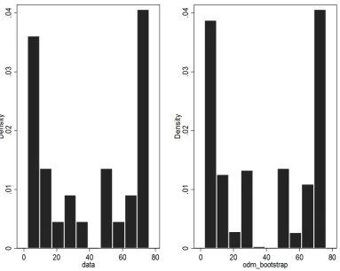
[image:7.595.115.499.416.722.2]

Based on the visual histogram (figure 4), which was used data set before and after bootstrap not really different in distribution. This visual histogram also shows that although the data point has been used, it is not deleted from the original data set in bootstrapping process. As a result, the same observation may be included in the resample data set.

The confidence interval for scalar parameters was calculated using percentile method to set approximate of bootstrap calculations. These refinements of the percentile method are the bias-corrected (BC) percentile method and the accelerated bias-corrected (BCa) percentile method. The 250 resample data sets had been used when calculating a BCa confidence interval. As a result of not having to calculate bias correction, a smaller value, in the range of resample data can be used when using the percentile method for estimating a confidence interval. As the number of resample data sets decreases, more variability is introduced into the confidence interval estimation.

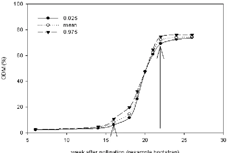
The 2.5% and 97.5% percentiles constitute the limits of the 95% confidence interval. The BCa method adjusts for bias in the bootstrapped sampling distributions relative to the actual sampling distribution, and is thus considered a substantial improvement using the percentile method. Based on this interval confidence (table 3), we known that week of 22 consistently produce the optimum oil content of palm mesocarp until week of 24 and 26. Those periods also give

coverage probability ≈ 95% and small variance, even though the range of interval confidence is little bit large.

[image:8.595.312.552.194.373.2]

For visual plot in Figure 5, we knew that the increases of oil content production after pollination were started from week of 16 until 21. The week of 22 consistently produce the optimum oil content of palm mesocarp until week of 24 and 26.

Table 3. Bootstrap: Interval confidence, range, and coverage of probability

Week Mean Varian LL UL Range Coverage of

probability 0.025 0.975

6 2.48 0.00 2.31 2.57 0.26 0.820

14 4.14 0.13 3.56 4.65 1.09 0.812

16 8.17 1.84 6.16 10.74 4.58 0.824

18 14.50 4.29 11.61 19.74 8.13 0.940

19 29.21 2.04 26.22 32.25 6.03 0.936

20 47.57 0.00 47.50 47.72 0.22 0.800

21 62.71 1.43 61.01 64.72 3.71 0.840

22 74.01 1.20 72.23 75.54 3.31 0.944

24 74.06 0.82 72.66 76.08 3.42 0.844

26 74.34 0.30 73.96 76.21 2.25 0.936

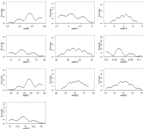
[image:8.595.120.494.410.659.2]

Silverman [12] proposed to try the bandwidth computed by replacing _R

( )

_f(v) _{in the optimal formula by R}

( )

_g (v)

σˆ where

g

σ is a reference density a plausible candidate for f,

and

_σ

_ˆ

2 _{is the sample standard deviation. The Silverman} formula had been done to find the optimum bandwidth of epanechnikov kernel. These bandwidths as a basic principal to build the optimum density of epanechnikov kernel distribution on resample data. As shown from the table 4 and figure 6, epanechnikov kernel has been successfully simulated the optimum estimate of oil content in palm mesocarp.

Plot estimation (figure 6) using epanechnikov kernel from resample bootstrap show that week of 22 produces the optimum oil content of palm mesocarp around 74% (ODM). This optimum consistently produces until week of 24 and 26. Based on this estimation, we can satisfy that epanechnikov kernel can be used to simulate the optimum estimate of oil

[image:9.595.311.552.112.274.2]

content in palm mesocarp.

Table 4. Epanechnikov kernel bandwidth

Week Bandwidth

6 0.0207

14 0.1192

16 0.4179

18 0.6593

19 0.4162

20 0.0115

21 0.3493

22 0.4637

24 0.2776

[image:9.595.70.536.308.729.2]

26 0.1681

5. Conclusions

In this paper, we have simulated the using of epanechnikov kernel as optimum kernel to estimate the oil content (%) of palm mesocarp at various periods. With respected to the method for finding optimal bandwidth. We propose Silverman [16] formula to determining the optimum bandwidth for epanechnikov kernel. The result show that epanechnikov kernel has been successfully simulated the optimum estimate of oil content (%) in oil palm mesocarp.

REFERENCES

[1] Efron, B. and Tibshirani, R. An Introduction to the Bootstrap, Chapman and Hall, New York. 1993.

[2] Davison, A. C. and Hinkley, D. Bootstrap Methods and Their Application, Cambridge University Press, Cambridge. 1997. [3] Hall, P. On the number of bootstrap simulations required to

construct a confidence interval, Ann.Stat.,14,4, 1453-1462. 1986.

[4] Shao, J. and Tu, D. The Jackknife and Bootstrap, Springer-Verlag, New York. 1995.

[5] Efron, B. Bootstrap methods: another look at the jackknife, Ann. Statist., 7, 1- 26. 1979.

[6] Efron, B. Nonparametric standard errors and confidence intervals, with discussion, Canad. J. Stat., 9, 2, 139 - 172. 1981.

[7] Efron, B. The Jacknife, the Bootstrap and Other Resampling Plans. vol 38, SIAM, Philadelphia. 1982.

[8] Efron, B. Better bootstrap confidence intervals, with comments, JASA, 82, 397, 171 - 200. 1987.

[9] Efron, B. and Tibshirani, R. An Introduction to the Bootstrap, Chapman and Hall, New York. 1994.

[10]M.P. Wand and M.C. Jones. Kernel Smoothing, Chapman & Hall, London. 1995.

[11]Rosenblatt, M. Remarks on some nonparametric estimates of a density function. Annals of Mathematical Statistics, 27, 832-837. 1956.

[12]Silverman, B.W. Density Estimation for Statistics and Data Analysis, London: Chapman and Hall. 1986.

[13]Wand, M.P. and Jones, M.C. Kernel Smoothing, London: Chapman and Hall. 1995.

[14]Wand, M.P., Marron, J.S. and Ruppert, D. Transformations in Density Estimation (with discussion). Journal of the American Statistical Association, 86, 343-361. 1991.