Stability Problems with Artificial Neural Networks and the Ensemble Solution

Stability Problems with Artificial Neural Networks and the

Ensemble Solution

Pádraig Cunningham1, John Carney1, Saji Jacob1,2

1_{Department of Computer Science, Trinity College Dublin, Ireland.}

2

Human Assisted Reproduction Ireland, Rotunda Hospital, Dublin 1, Ireland.

Abstract

Artificial Neural Networks (ANNs) are very popular as classification or regression mechanisms in medical decision support systems despite the fact that they are unstable predictors. This instability means that small changes in the training data used to build the model (i.e. train the ANN) may result in very different models. A central implication of this is that different sets of training data may produce models with very different generalisation accuracies. In this paper we show in detail how this can happen in a prediction system for use in In-Vitro Fertilisation. We argue that claims for the generalisation performance of ANNs used in such a scenario should only be based on k-fold cross validation tests. We also show how the accuracy of such a predictor can be improved by aggregating the output of several predictors.

1. Introduction

Artificial Neural Networks (ANNs) are hugely popular in research on medical decision support systems (see Baxt’s review of clinical applications of ANNs [2]). This is despite significant practical problems with their application. A practical problem that has come to prominence recently is that ANNs are unstable predictors. That is to say that small changes in the training data set may produce very different models [4][5][7] and consequently different performance on unseen data. Breiman suggests that these different models may result from the training of the ANN getting caught in different local minima in the error surface [5]. In this paper we show that this instability means that estimations of the generalisation performance of an ANN for a particular task may vary considerably depending on the training data used. We argue that, because of this, estimations of the generalisation performance of a single ANN should be based on a k-fold cross validation. Finally we describe how this instability problem can be fixed by building an ensemble of ANNs and aggregating the results of the networks in the ensemble to produce reliable predictions.

2. Learning from examples

The objective in using Machine Learning (ML) in medicine is to have the ML system learn to model a relationship that is represented explicitly in a set of historic data. The objective might be to learn the diagnosis associated with particular symptom combinations or likely treatment outcomes in particular situations. These are classification problems where the learning system learns to classify new examples into outcome categories or diagnostic classes. Alternatively the objective may be a regression task where the outcome to be predicted is a numeric value rather than a category – e.g. predicating chemical concentrations or determining dosage levels. There are many factors that influence the performance of such decision support systems applied to medicine. They have been proven to work best in ‘narrow domain’ medical fields where the cognitive span is narrow, an abstraction is available and hence prediction is amenable to structured queries [3]. Also the degree of representation of the biological/physiological process of the disease or medical event by those variables used in the machine learning algorithm influences the performance.

In any Machine Learning system the competence of the systems will improve with the amount of training data available. This competence (or accuracy) will follow a learning curve like that shown in Figure 1. Indeed the technical use of this term shares much in common with the vernacular use. Up to a certain point additional training data will produce appreciable increases in accuracy. However, beyond the knee point in the graph additional data produces little increase in accuracy. At the knee point the learning system has seen a useful cross section of data samples that represent a good coverage of the problem domain.

While this knee point will be clearly evident in a study such as that described in [20] it is very difficult to determine a priori the amount of training data that is required in a particular problem domain to give good coverage. The amount of data required for good coverage reflects the complexity of the input-output relationship being modelled (e.g. symptoms & diagnoses), the predictivness of the input features and the amount of noise in the data. All the nuances of straightforward problems may be represented in less than 100 examples but more complex problems may require several hundred or thousands of examples to provide good coverage.

Accuracy

Training Data Knee point

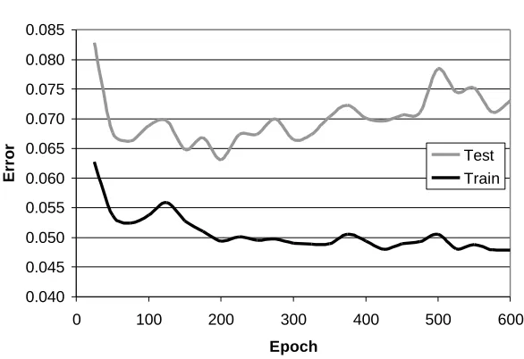
It is usually the case in studies of the use of ML in medicine that training data is scarce compared with the complexity of the problem being modelled. In that case the learning process is operating to the left of the knee point shown in Figure 1. Researchers often report that they expect the accuracy of their systems to increase with more data. A particular problem in developing ML systems with relatively small amounts of training data is that the training process may over-fit the training data. An example of this involving a Neural Net is shown in Figure 2 (a plot of error rather than accuracy). It can be seen that as the training of the network proceeds the error on the training data continues to drop but after 200 epochs (200 presentations of all the training data) the error on unseen test data starts to rise. After this point the network is overfitting to peculiarities in the training data and is loosing generalisation accuracy.

The standard solution to this problem is to hold out some of the available data from training and stop training when error on this validation set starts to rise. Unhappily, overfitting is more of a problem when data is scarce and using precious data in a validation set can ill be afforded. In situations where an abundance of training data is available, all the details of the problem will be well represented in the training data and overfitting is unlikely to be observed.

Average Train & Test Error

0.040 0.045 0.050 0.055 0.060 0.065 0.070 0.075 0.080 0.085

0 100 200 300 400 500 600

Epoch

Error

Test Train

Figure 2. This graph shows overfitting where error on unseen test data starts to rise after 200 epochs while training error continues to fall.(this graph is taken from an unpublished ANN model of

physicians’ prescription quantities of a certain drug).

2.1 Learning in an ANN

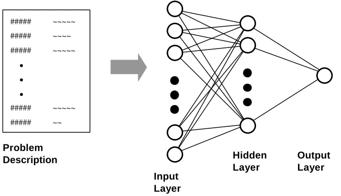
Figure 3 shows the structure of a feedforward neural network; the problem description is mapped to the input units (neurons) of the network and this input pattern is feed forward to produce the appropriate output.

For a numeric input pattern x=(x₁,...,x_i,...,x_n)

The activation on the jth unit in the hidden layer will be

∑

+ =

i ij i j

j f v xv

where f is the non-linear transfer function of the neuron – typically a sigmoid function. vijis a weight representing the strength of connection between input i and

hidden unit j. In turn the activation of the kth unit in the output layer will be

∑

+ =

j jk j k

k f w z w

y ( ₀ )

In the diagram there is only one output unit.

The network will have been trained by presenting problem descriptions and known outcomes to the network. The errors produced for the known outcomes will be used to adjust the weights in the network to reduce the error. The training process involves several thousands of weight adjustments until error reaches an acceptable level. The details of the training process will not be presented here but are covered in detail in [11] for instance.

##### ##### #####

##### #####

• •

•

~~~~~ ~~~~ ~~~~~

~~~~~ ~~

Problem Description

Input Layer

Hidden Layer

Output Layer

Figure 3. This diagram shows how a neural network may be used for decision support. When the problem description s mapped to the input layer of the network the appropriate output (classification or

prediction) can be read from the output.

For a given network architecture (i.e. number of units in each layer) the actual model of the decision making process that the network represents depends on the precise values of the weights v and w. The training of the network is a search through this weight-space to minimise error. Since the backpropagation training is a gradient descent process it may get stuck in local minima in this weight-space. It is because of this potential to get stuck in local minima that neural network models are unstable and high variance.

3. Evaluating the performance of an ANN for IVF

and the rest were symbolic. These features were all converted to a numeric form resulting in 53 inputs for the neural network.

It was determined that, with the training regime used, the neural network started to overfit after training for 250 epochs on average. In order to estimate generalisation performance 10 networks were built using 1305 data samples and tested using 50 data samples (25 positive and 25 negative). These produced the estimates of generalisation accuracy shown in Table 1. The average accuracy was 59%; i.e. the network was able to predict the outcome correctly for 59% of cases on average. However, because of the instability of ANNs this value ranged from 46% to as high as 68% across the 10 trials. So if this estimation of generalisation error were only done on one partitioning of the available data and we were lucky with the network we might be inclined to report an accuracy of 68% rather than 59%.

Table 1. 10 fold estimates of generalisation accuracy for the task of predicting outcome in IVF

Accuracy Estimates (10 fold) Average Min Max Std. Dev.

46 56 60 68 50 60 66 66 60 58 59% 46% 68% 7

In fact this evaluation of the use of ANNs in medicine using one partitioning of the training data (i.e. based on the performance of one network only) is quite common in the research literature. Systems have been evaluated in; auditory brainstem response analysis [21], in cancer screening [18], in trauma care [16], and in coronary risk assessment [1] for instance. It seems clear that because of the high variance of these estimates an evaluation on a single model is not adequate. If this model is retrained with new data it may have quite a different generalisation accuracy.

This need to use k-fold cross validation in evaluating ANN performance has been recognised by other researchers and applications using this methodology have been reported. The work by Kukar et al. [14] on diagnosing isachaemic heart disease uses 10-fold cross validation as does the work by Ulbricht et al. on analysing cardiotocograms [22]. Indeed Ulbricht et al. provide details of the range of performance they observe across the 10 networks and that analysis supports the findings presented here. Their set of 10 networks produces specificity figures (correct positives) between 72% and 90% and accuracy figures between 71% and 76%. This range of estimates of generalisation performance (particularly for specificity) illustrates the problem of instability highlighted in this paper.

3.1. High Variance in ANN outputs

not have. The first pair has accuracies of 56% and 62% resulting in a difference in accuracy of 6%. However, behind this figure, these networks disagree on 22% of their predictions. Similarly the next pairs disagree on 16% and 32% of their predictions. This disagreement reflects the instability or high variance of individual networks.

Table 2. Three pairs of networks with each pair tested on the same data may have similar accuracies but can disagree on several individual test samples.

Accuracy Disagree Accuracy Disagree Accuracy Disagree

1st Network 56% 60% 50%

2nd Network 62%

22%

56%

16%

62%

32%

The other point to note with these results is that the actual accuracy figures are very poor. Ironically, the disagreement of individual networks is a key requirement for improving performance by building an ensemble of networks and aggregating the results of these nets to produce improved results. Breiman has shown [6] that for unstable predictors, aggregating the output of several models will reduce variance and give more accurate predictions. Evidently there is no advantage in aggregating the results of a committee of experts if they all agree. In the final section of this paper an ensemble solution to the IVF problem is presented. It is shown that accuracy is increased significantly by aggregating the results of several networks.

4. The Ensemble Solution

Recently, ANN ensemble techniques have become very popular amongst neural network practitioners in a variety of ANN application domains. There are many different ensemble techniques, but the most popular include some elaboration of bagging Breiman [5], Freund and Schairpe boosting [12] or Wolpert stacking [23]. When applied to ANNs, ensemble techniques can produce dramatic improvements in generalisation performance -- see e.g. Carney and Cunningham [7] and Opitz and Shavlik [17]. The underlying idea of all these techniques is to generate multiple versions of a predictor, which when combined, will provide “smoother” more stable predictions.

Bagging (an abreviation of “bootstrap aggregation”) is one of the most popular ANN ensemble techniques. It uses the bootstrap Efron [10], a very popular statistical re-sampling technique, to generate multiple training sets and networks for an ensemble (see Figure 4 for an illustration of this). Although other ensemble techniques such as boosting have been shown to out-perform bagging on some data-sets Opitz and Shavlik [17], bagging has a number of key advantages when applied to real-world tasks such as medical decision support. One of the most important is the ease with which confidence intervals can be computed [8]. Another is the robustness and stability of the technique itself -- Breiman showed that it will always perform at least as well as an individual predictor, as long as the predictor is unstable [5].

disagreement amongst the ensembles compared to the individual ANNs in section 3.1. Also, the stabilising effect of bagging significantly improves overall generalisation performance.

Table 3. Three bagged ANN ensemble pairs with each pair tested on the same data.

Accuracy Disagree Accuracy Disagree Accuracy Disagree

1st Ensemble 61% 61% 53%

2nd Ensemble 64%

16%

63%

11%

69%

23%

Despite the attractive performance enhancing properties of ANN ensembles, there are surprisingly few examples in the literature that highlight their potential application in medical domains. An exception to this is the work of Lovell et al. [15], who applied their own variety of ANN ensemble to a pregnancy risk prediction task. Their results are also promising – their ensembles performed significantly better than individual ANNs and logistic regression techniques.

A variety of algorithms have been proposed to optimise the generalisation performance of ANN ensembles. In Carney and Cunningham [9] some important points relating to this issue are discussed in depth. Also, an efficient and robust technique for optimising the generalisation performance of bagged ANN ensembles is proposed and evaluated. For a comprehensive overview of other popular ANN ensemble techniques and issues related to training them effectively see Sharkey [19].

v

Train 0

Train 1

Train 2

Train n-2

Train n-1

ANN n-2 ANN n-2 ANN 2 ANN 1

Average Results

Result

ANN 0 Available Training Data

Train

5. Conclusions

This paper presents an overview of the instability problem with Artificial Neural Networks (specifically feedforward ANNs trained using backpropagation of error – these account for the vast majority of neural nets used in practise). This problem probably stems from the gradient descent training process settling in local minima. Different training conditions, such as small differences in training data or differences in network parameters, will result in the network stopping at different points in the weight space with resulting variations in performance.

One ramification of this is that estimations of generalisation performance based on a single network tested on data held back from training will have high variance. In section 3 it has been shown that another estimate based on a different partitioning of training and test data may produce a very different result. Thus estimations of training error should be based on k-fold cross validation testing.

6. References

[1] Azuaje F., Dubitzky W., Lopes P., Black N., Adamson K., Wu X., White J.A., Predicting coronary disease risk based on short-term RR interval measurements: a neural network approach. Artificial Intelligence in Medicine 1999;15:275-297.

[2] Baxt W.G., Application of artificial neural networks to clinical medicine. Lancet 1995;346: 1135-38.

[3] Blois, M. S., Clinical judgement and computers. New Eng. J. of Med. 1980; 303(4) : 192 –197.

[4] Breiman L., Heuristics of instability in model selection, Technical Report No. 416, Statistics Department, University of California at Berkeley, 1994.

[5] Breiman L., Bagging Predictors, Machine Learning 24 (1996) 123-140.

[6] Breiman L., Combining Predictors, in Combining Artificial Neural Nets: Ensemble and Modular Multi-Net Systems, A.J.C. Sharkey (ed.) pp 31-50, Springer, London, 1999.

[7] Carney J.G., Cunningham P., The NeuralBAG algorithm: Optimizing generalization performance in bagged neural networks, to be presented at 7th European Symposium on Artificial Neural Networks, Bruges (Belgium), 21-23 April 1999.

[8] Carney, J., Cunningham, P., (1999) Confidence and prediction intervals for neural network ensembles, in proceedings of IJCNN’99, The International Joint Conference on Neural Networks, Washington, USA, July,1999.

[9] Carney J.G., Cunningham P., Tuning diversity in bagged neural network ensembles, Trinity College Dublin Technical Report TCD-CS-1999-44, 1999.

[10] Efron B., Tibshirani R. An Introduction to the Bootstrap, Monographs on Statistics and Applied Probability, No 57, Chapman and Hall, 1994.

[11] Fausett L., Fundamentals of Neural Networks: Architectures, Algorithms and Applicants, Prentice Hall, 1994.

[12] Freund, Y., Schapire, R., Experiments with a new boosting algorithm, in Proceedings of the Thirteenth International Conference on Machine Learning, 148-156, Morgan Kaufman, 1996.

[13] Jacob S., Cunningham P., Carney J., Harrison R.F, Prediction of Assisted Reproduction Treatment Outcome using Artificial Neural Networks, submitted to Journal of Fertility and Sterility.

[14] Kukar M., Konenko I., Grošelj C., Kralj K., Fettich J., Analysing and improving the diagnosis of isachaemic heart disease with machine learning. Artificial Intelligence in Medicine 1999;16:25-50.

[16] Marble R.P., Healy J.C., A neural network approach to the diagnosis of morbidity outcomes in trauma care. Artificial Intelligence in Medicine 1999;15: 299-307.

[17] Opitz, D., Shavlik, J., Generating accurate and diverse members of a neural network ensemble, in: D. Touretzky, M. Mozer and M. Hasselmo, eds., Advances in Neural Information Processing Systems 8, 535-541, MIT Press, 1996.

[18] Ronco A.L., Use of artificial neural networks in modelling associations of discriminant factors: towards an intelligent selective breast cancer screening. Artificial Intelligence in Medicine 1999;16:299-309.

[19] Sharkey, A.J.C, Combining Artificial Neural Nets, Springer, London, 1999.

[20] Smyth B., Cunningham P., (1996) The Utility Problem Analysed: A Case-Based Reasoning Persepctive”, EWCBR’96 Advances in Case-Based Reasoning, Lecture Notes in Artificial Intelligence, I. Smyth & B. Faltings (eds.), pp392-399, Springer Verlag, 1996.

[21] Tian J., Juhola M., Gronförs T., Latency estimation of auditory brainstem response by neural networks. Artificial Intelligence in Medicine 1997;10:115-128.

[22] Ulbricht U., Dorffner G., Lee A., Neural networks for recognising patterns in cardiotocograms, Artificial Intelligence in Medicine 1998;12:271-284.