Hierarchical Production Planning in Make to Order
System Based on Work Load Control Method
Ehsan Fattahi
1,*, Mahta Khodadad
21Mazandaran University of Science and Technology, Iran 2Islamic Azad University, Firouzkoh Branch, Iran
*Corresponding Author: [email protected]
Copyright © 2015 Horizon Research Publishing All rights reserved.
Abstract
Subject to competition markets, continueschange in expectations, customer requisition and decrease of accessible production resource, the production system of make to order is the appropriate selection for response to today’s markets specifications and in order to provide the large spectrum of customer’s orders. In this research expend the control and planning production system (work load control) in make to order production system to manage the delivery time. For this, we recommend the hierarchical production planning structure. The major target is managing the activity in make to order system in order to achieve the short released time and entrance orders competition fee. To achieve this target we present the appropriate decision models with attention to restriction of production system. Finally due to consequent below: Present the expended release model to plain the production line and decrease the delivery time; Present the orders timing method in various stations. This method do subject to existences of previous level. Synchronistic performed the two methods state better performance in compare to others researches.
Keywords
Make to Order System (MTO), Make toStock System (MTS), Work Load Control (WLC), Hierarchical Production Planning (HPP)
1. Introduction
“Production Management Systems” (PMS) involves the need for a systematic look at the production. In absence of such a holistic look, production will be doomed to failure. Management of production, which is in a higher level than the production planning, is a way to implement a production schedule by managing all its components. In the above expression, the word “Management” is based on the fact that production planning is not instrumental alone, unless each component of the production schedule is managed and arrives at a result. Finally, the word “Production” is based on the experience that attention to production as an effective competitive weapon can anticipate firms relative to
competitors [1]. With this backdrop, we can say that PMS seeks with a holistic perspective and a proper planning to identify all effective elements and complexities of the production process to deliver a product on the market that increases customer satisfaction.
Today, manufacturing factories, considering the role of production in the competitive market system, find themselves in an environment totally changed. An example of this change can be observed in different industries of consumer goods and capital goods such as automotive, electronics, and appliances. A manager who is facing these rapid changes will have to adopt new approaches to address this competitive environment. Old strategy of integrated production planning has lost credibility and given itself up to the flexibility of new approaches. New approaches in production management have reduced the time required to designing and marketing products and the time between orders and their delivery to customers. Key features of new production environments include [2]:
a. Increase of product variety
b. Severe reduction of the product life cycle c. Change of social expectations
d. Change of patterns of costs
Considering these characteristics and to integrate themselves with new conditions, manufacturing firms must plan and manage different levels of their schedules so that they get the flexibility to confront unpredictable market changes.
the more it’s close to the beginning of production line, the stock of raw materials and semi-finished products is reduced and the product delivery time will be increased.
So far, several models of hierarchical production planning (HPP) in different manufacturing environments to improve the performance of manufacturing management were proposed. Kingsman et al. [13,14] have proposed a structure to manage orders which must be received by the make-to-order (MTO) system. In this case, some of the incoming orders are acceptance, and some of them are rejected. This stage in the MTO literature is called the order entry stage or customer inquiry stage. In this model, entry process is divided in two phases: the client application and the order entry system. Cakravastia et al. [15] was assuming that the order has been accepted by the customer, price and delivery time should be determined through talking between the customer and suppliers. Caloso et al. [16,17] provided the decision making structure for negotiation between customers and suppliers in the supply chain. In these articles, three correct number linear models have been proposed to select the suppliers and orders which have highest profits for the company. Breithoupt et al. [18] determined the sensitivity of the HPP structure to parameters such as workload high limits and time horizon and identified critical parameters. Then, a new method for calculating these parameters were presented to improve the output of the HPP structure. Rabbani et al. [19,20] proposed the HPP structure for combined MTS/MTO environments. As a novelty of this research in comparison to the literature review, the HPP structure was proposed in four levels.
2. Make to Order (MTO) System
In these environments, CODP precedes the production process of semi-finished products. Composites are designed and manufactured according to customer demand. Product selection in MTO production environments is made by customers. The implementation of an environment which engages in production only after the customer orders are received where all workstations produce only the raw materials required for the completion of customer orders, and where the stock of raw materials in all workstations are very low even zero, a coordination is vital between different levels of the factory, reduced time of supply, high flexibility of the production line, and use of complicated and expensive equipment. The planning of such production systems is a difficult and complicated task [3].
3. Hierarchical Approach of Production
Planning in Production Management
System
Given the major defects of the integrated approach, this perspective will not be a good solution to manage production in today's organizations. In general, planning and control of
production and raw materials is not a single activity that can be managed by the integrated approach. By cons, it depends on a series of decisions about various topics in the production system. These decisions are taken generally in different levels of management according to the hierarchy of production activities, so that any compliance with this hierarchical structure of decision-making will tighten the horizon of decisions but will increase the details of the data needed to make decision. To better manage various activities of production, a close relationship between the decisions taken at successive levels is necessary.
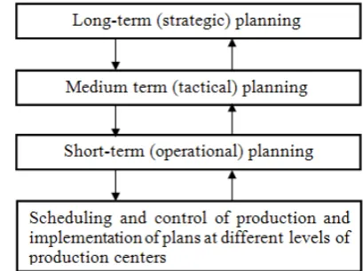
Hierarchical Production Planning (HPP) is an effective method to perform this multilevel process of hierarchical decision-making. In this hierarchical approach, the main problem of decision-making is decoupled into sub-problems at different levels of decision-making; then these sub-problems are solved in a given sequence according to the different levels of hierarchical structure. Also, to maintain the integrity of the main problem and the interconnection of these sub-problems, the response at each level of the hierarchical structure will be considered as a limitation in the decision-making model at a lower level [4].
[image:2.595.326.531.372.525.2]In general, a bottom-top feedback mechanism is used in a HPP structure to improve decisions made at higher levels [5].
Figure 1. Hierarchical Structure of Decision-Making in Production Management
4. Structure of the Proposed System of
Planning and Production Control
(WLC) in MTO Production
Environments
Work load control (WLC) is an improved approach used to have a successful system of planning and production control in MTO production environments with respect to the hierarchical approach. In other words, we propose in this paper a hierarchical structure of WLC in order to better control the activities that affect the delivery time of customer orders.
four different levels of planning.
4.1. First Level - (Customer Enquiry Stage)
In this stage, given the demands of the customer, we check if MTO firm is able to meet the demands of a customer given the limitations of the system, new orders, and degree of signification of the customer. The output of this level of WLC is to accept or reject orders.
4.2. Second Level - (Order Entry Stage)
In this stage, if the customer’s orders are not rejected at the first level, three final decisions will be made:
a. Determine the price and delivery time of new orders (delivery is determined only if it is negotiable). b. Plan the ability to accept new orders.
c. Choose a group of contractors who are able to provide necessary raw materials for new orders in a timely manner and a reasonable price.
4.3. Third Level – (Release of Orders into the Shop Floor)
This stage includes only accepted orders for which raw materials are available (output of the second level). In this stage, given the delivery time of orders and also the density of the work in different workstations, delivery of new orders in the system will be permitted.
4.4. Fourth Level – (Prioritizing Orders in Workstations)
In this stage, orders awaiting delivery in workstations are given priority so that their delivery time is minimized.
For a better communication and improved efficiency of the production system, feedbacks are taken into account from lower to higher levels.
5. Distinguishing Features of the
Research
The distinctive features of this research compared to other researches carried out in this area are as follows:
a. Consider the significance level of customers to decide whether to accept or reject new orders by appropriate analytical tools.
b. Introduce a new structure of decision-making to accept or reject orders at the first level and determine the delivery time and the price of incoming orders at the second level, by an integer mathematical model. c. Consider all components of the supply chain in the
delivery and price control including customer MTO firm and contractors to reject or accept orders received at the MTO system.
d. Offer alternatives to determine the delivery time of entry orders and thereafter, different prices for these
orders, and facilitate the negotiation process between customer and MTO system are the most difficult stages of decision-making to reject or accept orders. e. Select contractors to perform works related to new
orders received in the system at a given price and delivery time by an integer mathematical model of planning.
f. Extend the process of order release into the shop floor to access the shorter delivery time and improve the efficiency of production line by reducing the density of works according to WLC perspective.
6. Delivery Time Components in MTO
Systems
Delivery time components in MTO production environments include the following:
a. Negotiation Time (NT): The time between the arrival of an order (customer request) and the decision on its acceptance or rejection.
b. Raw Material Lead Time (MLT): The time between putting in an order for raw materials needed and the time of its acceptance.
c. Product Delivery Date (PDT): The time of entry of raw materials into the system, namely, when orders are ready to be released. These kinds of orders are placed at the warehouse specified for orders to be released. The waiting period between the entry of raw materials and the time of their delivery into the production system is referred to as waiting period in the warehouse of orders to be released.
d. Order completion date in the shop floor (SFTT): The time between the release of orders into the production system and delivery of customer orders.
Total Time Manufacturing (TMT) includes SFTT and PDT. Finally, the Due Date (DD) which includes the total TMT, MLT and NT.
Equation (1-3) shows how to calculate the TMT and DD.
TMT
MLT
NT
SFTT
PDT
MLT
NT
DD
PDT
SFTT
TMT
+
+
=
+
+
+
=
+
=
...
7. Variables Examined in this Study
7.1. Dependent Variables
a. Costs of a production system include the costs of production variables in normal time, overtime, sub-contracting, and the costs of postponed orders where delivery delay is permissible.
7.2. Independent Variables
a. Total capacity of workstation r including normal time, overtime and sub-contracting assigned to order i in period t.
b. A certain capacity of workstation r assigned to order i during overtime.
c. Degree of delay in delivery of order i in due date. d. Order i completion Date.
e. A certain capacity of workstation r during overtime is assigned to order i.
8. First Level of the Proposed WLC
Approach: Customer Inquiry Stage
At this level of the proposed structure, we will discuss the question of accepting or rejecting new orders. This decision is based on three main criteria including total capacity available during planning, customer significance level for the organization, and order characteristics such as the workload required on the production line.
This model is divided into two levels depending on order delivery time. The first level consists of two steps: In the first step, incoming orders are grouped according to the number of customers who made an order. In the second step, the ability of production system and all orders are generally compared to see whether new orders can be completed within the planning horizon. If the current capacity can meet new orders, the orders enter into the second level; otherwise, other decisions are made. The steps mentioned in the first level are the same for both types of orders with negotiable and fixed delivery time.
8.1. First Step - Grouping Incoming Orders According to Customer Significance for the Organization
Group 1 - The organization completes customer orders in the best condition.
- Fixed and long relationship with the organization.
Group 2 - The competition between different manufacturing organizations to boost customer satisfaction.
- Improving the functioning of the organization leads to increased sales.
Group 3 - Casual orders
- Weak relationship and lower ability to deliver orders at due date.
Group 4 - Irregular and small amounts of purchases
8.2. Second Step - Capacity Estimated Calculation
In this step, each time a new order comes in, the sufficiency of current capacity is considered within the planning horizon at the first level. To this end, estimated calculation is performed as follows:
1. If an order is highly significant, the following relation is used to estimate the capacity thereof:
(
t
T
)
t
r
C
p
TWK
now
rt O
i r ir i
...,
,
,
;
)
(
=
∀
≤
×
∑
∈
i: Order index
r: Workstation index
Or: All orders needed in workstation r
t: Planning period index
tnow: Time now
T: Length of planning horizon at the first level
Crt :Maximum capacity of workstation r in period t including normal time, overtime, and sub-contracting.
TWK
ij : Workload required by the order i in workstation j.P
i: Possibility to accept order i put in by a customer.During the entry of a new order, three kinds of order exist in the output system: orders approved by the customer and all of which are released in the production system (RO); orders approved by the customer which are not yet released in the production system and are planned to be backlogged (PO). The third kind of order is contingent order (CO) in which delivery time and price are determined by the production system, whose approval or cancellation is not yet decided by the customer. The new order is of the third kind. Contingent orders may be finally canceled by the customer. Pi-value for orders approved by the customer (RO and PO) is 1. For other orders (CO) which are not yet canceled or accepted by the customer, this value will be 0 or 1 using previous data and experiences of marketing and sales unit.
If for the new order, which is highly significant, there is not sufficient capacity in some workstations, the following alternatives are suggested for decision making about the order:
a. Increase the capacity of production system to prepare a new order: due to the significance of the new order in workplaces where there is not sufficient capacity within the planning horizon T, basic decisions are taken by management to increase the capacity. b. Delay certain orders in the system that are of medium
significance: in this alternative, we examine whether the delay in preparation of some orders of medium significance gives us the possibility to complete them at the planning period.
c. Cancel orders that are unimportant (or of low significance) and are not yet approved by the customer (contingent orders). This way we will have the capacity to complete the new order.
d. Reject the new order: the new order can be rejected if its completion requires considerable additional capacity which is unavailable.
(
t
T
)
t
r
C
p
TWK
now
rt rt
O
i r ir i
...,
,
,
);
1
(
)
(
=
∀
−
×
≤
×
∑
∈
α
αrt is a percentage of total Crt capacity that is considered for highly significant orders in future. This value is determined by the management of organization according to future orders forecasted by sales and marketing unit. If the above equation is not established, decision making on this order will include the following cases:
a. Delay new orders of medium significance: This alternative can be used only when the delay of an order allows its fabrication within the planning period T. b. Rejecting a new order of low or medium significance:
In case the completion of a new order requires considerable additional capacity which is unavailable, this order may be rejected.
c. Delay some PO and RO with medium significance: At manager’s discretion, some PO and RO with medium significance can be postponed to create sufficient capacity for new orders.
9. Second Level of the Proposed WLC
Approach Order Entry Stage
The second level of the proposed structure includes determining the delivery (if unspecified) and price of orders arrived in the production system according to various limitations and inside and outside of organization. Two main criteria for deciding the acceptance or rejection of new orders is their price and delivery time. These two criteria are highly interdependent. If the delivery time is short and compact, in addition to normal production time, production system shall adopt other policies, including overtime, delaying other orders in the system, employment of new staff and sub-contracting to complete the order. All these policies impose costs on the firm and affect the cost price of new orders.
The second level consists of four steps. If the order is not rejected at the first level and if the delivery of the new order is fixed, we use backward method in the first step of the second level to calculate the latest or earliest release time inside the production system. These times will be compared to the average delivery time and the workload required by contractors to make appropriate decisions.
In case delivery time is negotiable, there will be suitable alternatives to create different delivery times. If an order is accepted in the first stage, we use a mathematical planning model in the second stage that we call IP1 to calculate the price and delivery time.
As for orders with stable delivery time, cost price will be announced to the customer, and for orders with negotiable delivery time, the delivery time will be made known to the customer in addition to the price. In the third stage, the
customer compares these data with those from other MTO firms and takes into account its own criteria to determine the rejection or acceptance of the order. In the fourth stage, a good group of contractors will be selected by a mathematical model of planning (IP2) to perform the workload required for the delivery of accepted orders.
Since the implementation of the second and fourth stages is time consuming because of the use of integer mathematical models, these stages are completed according to the following conditions:
a. A significant order enters the system.
b. When the number of new orders arrived in the system exceeds a certain limit.
c. When the difference between the time the first order comes in exceeds a certain limit after completion of the second stage.
9.1. Deciding on Rejection or Acceptance of Orders with a Stable Delivery Time
If a new order has a stable delivery time, the status of the new order will be determined in four stages:
a. Create different alternatives to calculate the price of the new order
b. Resolve the integer linear model (IP1) to determine the price of the new order
c. Decide to accept or reject the order by the customer d. Select contractors to provide raw materials and
required workload to complete the new order. 9.1.1. Creating Different Alternatives to Calculate the Price
of the New Order
After considering the estimated capacity to determine if an order can be completed within the planning horizon of the first level, we engage in first stage of the second level. To run the integer planning model (IP1) and determine the price of the new order, it is necessary to specify the input parameters of the problem including Order Completion Date (OCD) at each workstation, Earliest Release Date (ERD) and Latest Release Date (LRD). If the order is sent into the system after LRD, it will not be possible to complete the delivery at due date.
Since delivery time is not known, the backward method is used to calculate the OCD and ERD. In previous research, the following formula was used by Kingsman et al [5]. to calculate OCD and ERD:
, ( , )
, ( , 1) , ( , ) , ( , )
, ( , ) , ( , 1) , ( , 1)
, ( ,1) , ( ,1) i i ni
i i ni i i ni i i ni
i i r
i
p
i i r i i r p
i i i i i p
i i
OCD
dd
OCD
OCD
TWK
W
OCD
OCD
TWK
W
LRD OCD
TWK
W
ERD LRD pool delay
µ
µ µ µ
µ µ µ
µ µ
−
+ +
=
=
−
−
=
−
−
=
−
−
ni: Number of workstations on the operational route of order
i
µ(i,r) :Workstation r on the operational route of order i
ddi: Delivery time of order i
Crt: Order i completion date in resource r
Pool delay: Total workload of all PO orders
p
W
: ting d in each workstation for one work of priorityp.p includes both normal and high priorities.
For orders of medium and low significance, normal priority is taken into account, but for orders of high significance, in addition to the normal priority, if delivery of the order is not possible at dd, we can complete the order by reducing the (high priority) waiting period. Due to the capacity limitation of the temporal warehouse of workstations, a percentage of orders of high significance can be given high priority. Wp can be calculated by the following equation :
R
TWK
T
Wp
Rr i Or ir
′
−
=
∑∑
= ∈1)
(
In the above equation, R' is the average number of workstations to complete an order.
Order completion date in a workstation is determined by reducing the waiting period (Wp) and workload required by the order (TWK) from order completion date in the next workstation. This formula can determine relatively accurate dates for ERD and OCD only when there is sufficient capacity in each workstation.
In addition to the above equation, the following is presented for the first time given the capacity of individual workstations:
delay
pool
LRD
ERD
ST
LRD
ST
OCD
B
P
TWK
ST
OCD
ST
OCD
B
P
TWK
ST
OCD
ST
OCD
B
P
TWK
ST
OCD
dd
B
P
TWK
ST
OCD
i i i i r i n i i n i i n i n i i n i i n i i i n i n i i n i i n i i i i i i i i i i i i i i r i i r i i r i i r i i r i i i i i i i i i i−
=
=
≤
+
×
+
=
≤
+
×
+
=
≤
+
×
+
=
=
+
×
+
=
+ − − − − − ) 1, ( , ) 2 , ( , ) 1, ( , ) 1, ( , ) 1, ( , ) 1, ( , ) 1 , ( , ) , ( , ) , ( , ) , ( , ) , ( ,;
;
;
1 ) , ( , ) 1 , ( , ) 1 ( ) 1 , ( , ) 1 , ( , ) 1 , ( , ) , ( , ) , ( , ) , ( , µ µ µ µ µ µ µ µ µ µ µ µ µ µ µ µ µ µ µ i rST
: Is the earliest time when workstation r has thesufficient capacity to complete the order i. This time, in the example of the previous page, is the third day of the ninth week. Order completion date in the previous workstation is less than or equal to that date, which is written as an “unequal” in front of each equation.
r
B
:
Is the waiting period at workstation r before thenecessary operation is accomplished in this station on the new order. Queuing at each workstation is separated into two parts:
a. Queue of order with normal priority: In this status, the new order is placed at the end of the queue in each workstation.
b. Queue of order with high priority: This queue consists of two parts: One is for orders of medium and low significance, and the other for orders of high significance. The first part precedes the second. The stage where a high priority is given to new orders is described below.
Because of capacity problems, calculated values of OCD and ERD will be more accurate and the possibility of a reliable delivery time will be increased. In addition to capacity, the calculation time necessary for the orders according to the possibility of their acceptation (P) is a further advantage of the proposed formula.
Prior to the implementation of IP1 model (second stage), it is necessary to compare the Raw Material Arrival Date (MAD) by contractors and LRD and ERD values to ensure that it is possible, considering the MAD, to complete the new order at due date. At first and second level of the proposed WLC approach in MTO systems, medium term planning system is made and we do not need more accurate data. We only calculate an average value of MAD according to the performance of contractors in the past. Where raw materials arrive on time into MTO system, there is no need to prioritize or make other additional works including overtime and sub-contracting, and the order will be placed at the end of the queue of orders to be released. Otherwise, if raw materials do not arrive to the firm at due date, the following solutions are proposed for better decision-making and management of new orders. To this end, tnow
,
LRD, ERD and MAD values will be compared. The following status will occur when comparing these values:A- LRDi<tnow
:
In this case, it is not possible to complete the order at due date, and it is better to reject the order.B- ERDi <tnow<LRDi
:
Under such conditions, it is not possible to complete the order in a normal status. The order(MAD-ERD) will be completed with delay (assuming that
this order is at the end of the queue of orders to be released). Here are the alternatives proposed to deliver the order at due date:
shorter delivery time. This reduction will allow this relation ERD = MAD to be established. This reduction also increases the priority of orders waiting to be released. In other words, in this alternative, the order is given a higher priority at least to the point of MAD - ERD. The new value is equal to Pool Delay:
MAD LRD
y
Pooldela ′= i −
2) Change in OCD values: Change of OCD in different workstations is another way to reduce delivery time. This change can be performed by three ways:
a. Changes in the values of OCD for a new order by increasing the capacity of workstations: In this status, all workstations that are necessary to accommodate the new order are considered and, in case of increased capacity, new OCD values will be calculated. The change in OCD values should be calculated as the new ERD is equal to MAD. This alternative does not change the OCD for other orders in the system.
b. Changes in the values of OCD for a new order through changing the OCD for other orders: Orders where ERD is greater than MAD, it is likely to change the values of OCD, without their delivery time is altered. By changing the OCD values for other orders, capacity for the new order will be increased; with this new capacity, OCD values of the new order will be reduced and, subsequently, ERD will also be reduced. Raw materials required for orders where ERD is greater than MAD will be entered into the system before due date and, therefore, we need to keep the raw materials in the relevant warehouse. This alternative will reduce the waiting period for raw materials needed by such orders and, therefore, the cost of raw materials warehoused will be reduced, which is one of the goals of MTO systems.
c. Changes in OCD values using the capacity assigned to other orders: by assigning the capacity for orders in the production system, it is possible to achieve a new order where ERD value is less than that of MAD, thereafter, reduce the values of OCD in individual workstations and accelerate the delivery. This alternative changes the OCD values where additional capacity for the new order is created. Using the capacity assigned for these orders will delay their delivery. This additional capacity will be calculated so that the new ERD is at least equal to MAD. This alternative is used for new orders of high significance.
3) High priority in the queue between different sources of production: Giving high priority to a new order, it will be possible to reduce the waiting period and thus delivery time. High priority for orders of low significance include placing the new order at the end
of the queue of the first part, and for orders of high significance include placing the new order at the end of the queue of the second part. Reducing waiting period in different workstations shall be such that the relation ERD = MAD is established.
4) Lateness: If possible, orders can be completed behind schedule. This alternative is only possible for orders of less significance.
5) If it is not possible to use such alternative and if there is no other suitable solution for the delivery of the new order at due date, the order will be rejected at the discretion of management.
It is also possible to use a combination of these alternatives to complete the order at due date.
C- tnow<MADi<ERDi:
Raw materials are delivered on time and the order is placed at the end of the queue for orders waiting to be released.
D- ERDi <MADi <LRDi: This status resembles the status (B).
E- MADi > LRDi:
In this status, MAD is later than LRD. Here, it is difficult to prepare the order on schedule and it is highly possible that the order is postponed. All such alternatives of the second part are also available in this status, with the difference that the level of reduction of delivery time will be so that MAD and LRD values are equal.
9.1.2. Resolving the Integer Linear Model (IP1) to Determine the Price of the New Order
At the first level of hierarchical production planning model, integer linear model is used to calculate the price of incoming orders where the delivery time is specified. If the order is not rejected by the MTO system in the second stage, in this stage, an integer linear model is used to calculate various costs imposed on the system because of the new order. Final price of the order is calculated by totaling costs. As in the previous stage various OCD and ERD values were calculated by different alternatives, therefore, IP1 model was applied in exchange for each set of values (OCD and ERD). In addition, the lowest price of the order will be announced to the customer. The optimal value (OCD and ERD) is chosen for each optimal response at IP1 model. Indexes, parameters and variables of the decision taken by the IP1 model are listed
:
Indexes:
i: Order index (i=1,...,n) r: Workstation index (r = 1, ..., R)
t: Time index (t=1,...,T)
Input parameters:
cr irt: Manufacturing cost of order i in workstation r in normal time and period t
cs irt: Manufacturing cost of order i in workstation r by contractor in period t
ct
i: Cost of delaying the order i per unit of timeiwpr: Total workload for orders behind the schedule
iwirt: Total workload of order i in workstation r with a ST time in period t (coming into the system)
owirt: Total workload of order i in workstation r with an OCD in period t (coming out of the system)
CRrt: Maximum capacity available in workstation r in normal time and period t
αrt: A percentage of CRrt total capacity is taken into account for orders of high significance.
COrt: Maximum capacity available in workstation r in period t during overtime
CSrt: Maximum capacity available in workstation r in period t by contractors of the firm
OS(i): All orders that are completed on time.
M
:
A very large number. Decision variables:Yirt: Total capacity in workplace r including the normal time, overtime and sub-contracting assigned to order i in period t.
Oirt: A certain capacity of workstation r assigned to order i during overtime.
Sirt: A certain capacity of workstation r assigned to order i by contractors.
LT
i:
Delay of delivery of order iFT
i:
Order i completion date0
), , (,µ in t
>
i i
Y
Otherwise
x
it=
0
[
]
1 1 ( )
(
)
. .
(1)
(
)
(1
);
,
(2)
;
,
(3)
;
,
r
r
r
r
R T
irt irt irt irt irt irt irt irt i i
i O r t i OS i
irt irt irt rt rt i O
irt rt i O
irt rt i O
MIN Z
cr
Y
O
S
co
O
cs
S
ct LT
S T
Y
O
S
CR
r t
O
CO
r t
S
CS
r t
α
∈ = = ∉ ∈ ∈ ∈=
×
−
−
+
×
+
×
+
×
−
−
≤
× −
∀
≤
∀
≤
∀
∑ ∑∑
∑
∑
∑
∑
{ }
0
,
1
;
,
(
)
&
0
,
)
13
(
,
,
;
0
,
,
)
12
(
)
...,
,
1
(
,
),
(
,
;
)
11
(
)
(
;
)
10
(
)
(
);
(
)
9
(
)
(
,
);
1
(
)
8
(
),
(
,
;
)
7
(
)
...,
,
1
(
,
),
(
,
;
)
6
(
,
;
)
5
(
;
)
4
(
) ( 1 1 1 1 ), ( 1 ), ( 1 1 1 ), , ( ,i
OS
i
t
X
FT
LT
O
i
t
r
S
O
Y
dd
t
O
i
i
OS
i
r
Y
p
ow
i
OS
i
dd
T
LT
i
OS
i
dd
FT
LT
i
OS
i
t
X
M
t
FT
i
OS
i
t
X
M
Y
dd
t
O
i
i
OS
i
r
Y
p
iw
t
r
Y
p
ow
r
Y
p
iw
iwp
it i i r irt irt irt i r dd T t k irk tk irk i i i i i i it i it i r t k irk i t k irk O i OS i i
t k irk O
i OS i i
t
k irk i O
i i O
The objective function of the model consists of minimizing the production system’s costs including the costs of production variables in normal time, overtime and sub-contracting, and also those for postponed delivery of orders that may be completed behind schedule. By resolving the IP1 model, main components of the new order’s cost price will be determined including all costs of production variables and postponed delivery of orders that may be completed behind schedule due to the addition of new orders. Given the necessary workload that must be acquired from contractors and the benefit that is determined by management, we can calculate the cost price of the new order. Limitation (1): Limited capacity in normal time; limitation (2 and 3): Limitation of maximum time for overtime and sub-contracting; limitation (4): This limitation guarantees that all input works are completed within the planning horizon T. Only the limitation (4) does not guarantee if orders can be completed at due date, because OCD takes place at different periods within the planning horizon of the first level. Limitations (5 and 6): These limitations are about orders to be completed at due date. Application of limitation (5) helps the completion of orders in different workstations at their relevant OCD. This limitation increase the possibility of order completion at due date. Planning at first level is performed weekly. An OCD may be on third day of the week. Application of this limitation (5) simply guarantees that the order will be completed at the end of a week. To make sure that the order will be completed exactly on the third day of the week, limitation (6) is applied. This limitation is considered only for orders of high significance that must be completed at due date. In other words, the limitation (6) guarantees that the remaining work related to the order shall be completed in period t on due date. In limitation (7), OCD is calculated at the final workstation. This time is saved by taking the binary value of (Xit =1)Xit. By application of
this limitation (8), OCD is calculated. In limitation (9), this time is compared with the promised delivery time to calculate the delivery delay. Limitation (10) ensures that the maximum delay of any order is to the extent that the order will be produced within the planning horizon. Limitation (11) is similar to limitation (5) with this difference that, here, OCD may be delayed (LTi). In other words, limitation (11) ensures that the amount of work remaining until period t for orders that are delayed should be completed in the time interval between t and ddi+LTi. This limitation causes that sufficient capacity for timely delivery of orders is released. Limitations (12 – 13) are nonnegative limitations to make sure that decision variables are correct.
9.1.3. Deciding to Accept or Reject An Order by the Customer
A new order’s price is determined by implementing IP1model. This price is announced to the customer. If the customer approves the order to be completed at MTO firm, the firm will perform necessary actions in the next stage by providing necessary workload and raw materials through contractors.
9.1.4. Selecting Contractors to Provide Raw Materials and Required Workload to Complete New Orders
The question of selecting a set of contractors to provide necessary workload for accepted new orders is the last stage of the suggested structure. Criteria for contractor selection are price and delivery time. As mentioned before, in exchange for various alternatives, each of which contains their own ERD and OCD, IP1 model is implemented and, finally, the lowest price offered is chosen. IP1 implementation has an ERD and OCD value in different workstations in exchange of which the lowest price is obtained.
Given the output of the IP1, if MTO firm is obliged to use contractors to provide new orders’ workload and ensure their delivery time, it is necessary that some of the existing contractors are chosen.
STirtimes at the second stage of the proposed structure are calculated.
STir is the latest time that necessary operation is commenced in workstation r regarding order i.
If necessary workload for order i which is provided by contractors enters production system after this time, it will not be possible to get a pre-calculated OCD. Since it is possible that some specified or unspecified orders are rejected from the time these values are calculated to the implementation of IP2 model, STir values should be recalculated and updated.
In this stage, the objective is to determine a set of contractors who offer the least delivery time difference with respect to STir values, and suggest a lower price to provide necessary workload. IP2 model is suggested to find this set of contractors.
According to requirements of orders whose fabrication has been newly accepted in the system, the necessary amount of raw materials and workload are provided by contractors. Therefore, the amount of raw materials and workload are already known. In other words, IP2 is an allocation model in which given the criteria of price and delivery time some of the contractors available in the present set are selected. Unlike IP1 model, IP2 model is applicable only for orders that are accepted by the customer and their production has been ensured. Orders that have not been yet approved by their customer can cause raw materials and workload to be ordered more than needed. This also may impose many costs on MTO systems. After the new order price is announced to the customer, a time shall be spent by the customer to perform the negotiating process and confirmation of the order. During this time, some of the orders that were not still approved by the customer in the IP1 model may be approved before a new order is confirmed by the customer in IP2 model. It is assumed in IP2 model that workload required by an order in a workstation can be provided only by one contractor.
Indexes:
Input parameters:
STir
:
The latest time that necessary operation is commenced in workstation r regarding the order i; otherwise, the order will be postponed.Pirs
:
Suggested price of contractor s to deliver the required workload for the order i in workstation r.MADirs
:
Delivery time of the required workload for the order i in workstation r by contractor s.Sirst: Maximum amount of workload for the order i in workstation r thatcontractor s can provide in period t.
βir
:
Penalty for the arrival of necessary workload of order iin workstation r prior to schedule.
β'ir
:
Penalty for the arrival of necessary workload of orderi in workstation r behind schedule. Considering that the late
arrival of raw materials and, consequently, late delivery of orders may impose many costs on the firm, the amount of the delay should be so that raw materials enter the firm on or prior to schedule (βir
>>
β'ir).NO(i)
:
Set of new orders accepted.L'(i)
:
Set of contractors who can deliver the workloadrequired by order i in workstation r before their Stir.
S(ri)
:
Set of contractors who can deliver the workload required by order i in workstation r.Decision variables:
Xir = 1, if workload for order i in workstation r is provided by contractor s.
Otherwise, Xir = 0
1 1 ( ) ( ) 1 ( )
( ) 1 ( ) 1 1 1 ( )
(
)
(
)
(
)
(
(
))
i
i i
I R R
irs irs irst ir ir irs irs
i r s S r i NO i r s L i
R R T
ir irs ir irs irt irt irt irst irs irt irt
i NO i r L k i r t s S r
MIN Z
P
X
S
ST
MAD
X
MAD
ST
X
cr
Y
O
S
X
co
O
β
β
′
= = ∈ ∈ = ∈
′
∈ = ∉ = = = ∈
′ =
×
×
+
×
−
×
′
+
×
−
×
+
×
−
−
×
+
×
∑∑ ∑
∑ ∑ ∑
∑ ∑ ∑
∑∑
∑
I
∑
1 ( )
(1)
(
(
(
))
(1
);
,
i I
irt irt irst irs rt rt i s S r
Y
O
S
X
CR
α
r t
= ∈
−
−
×
≤
× −
∀
∑
∑
1
(2)
I irt rt;
,
i
O
CO
r t
=≤
∀
∑
1 1 1 1
(3)
r I T irt I T irt;
i t i t
iwp
iw
Y
r
= = = =
+
∑∑
≤
∑∑
∀
( ) 1 1 1
4
;
,
( )
I t irk I t irk OS ii k i k
r t
ow
Y
∈ = = =
=
∀
∑ ∑
∑∑
1 1
1 1
( )
(5)
;
,
( ), (1,...,
)
(6)
;
,
( ), (1,...,
)
(7)
1;
,
( )
(8)
,
0;
; , , ,
( )
ii
t t
irk irk i
k k
t LT t
irk irk i
k k
irs s S r
irt irt irs i
iw
Y
r i OS i t
dd
ow
Y
r i OS i t
dd
X
r i NO i
Y O
X
i r t s S r
= =
+
= =
∈
≤
∀ ∈
∈
=
∀ ∉
∈
= ∀ ∈
≥
∀
∈
∑
∑
∑
∑
The objective function of IP2 model includes different costs of manufacturing an order plus the costs for purchasing raw materials and workload from contractors and the penalty for delivery prior or behind schedule by contractors. In IP2 model, input parameters include the following: necessary amount of workload and raw materials to be provided by contractors, and also raw materials’ delivery time before running the model. As previously mentioned, IP2 model only applies to orders confirmed and approved. Therefore, the value of such orders is 1 in IP2.
Limitations (1 – 6) are similar to IP1 problem limitations, but they are only for approved orders. Limitation (7) guarantees that the necessary workload regarding an order in a workstation may be provided just by one contractor. The application of IP2 model only for approved orders will update data and parameters at the first level. In other words, fifth stage indicates the modality of implementing the rolling horizon approach for the first level of hierarchical production planning structure.
By implementing IP1 and IP2 models, one the one hand, the order is completed with the least possible cost and it is more likely acceptable by customer; one the other hand, a group of contractors are selected who will provide necessary workload and raw materials at the lowest possible cost and at the latest period. MTO manufacturing firms have an appropriate and effective relation with different components of supply chain which plays a major role in the effective performance of MTO systems; it also creates a flexible production schedule which complies with internal and external limitations in order to earn greater profits. This
planning method can facilitate release and scheduling of orders at low levels of planning.
9.2. Deciding to Reject or Accept Orders with Negotiable Delivery Time
In this status, no fixed time for order delivery is offered to the firm by the customer, but it asks the firm to offer a combination of delivery time and price so that it makes its decision according to its own criteria. In this case, similar to fixed delivery time, four main activities are carried out that are as follows:
B (1) – Production of various alternatives to calculate the delivery time for new orders
B (2) – Determining delivery time and price of new orders by implementing integer linear model (IP1)
B (3) – Deciding to reject or accept orders through negotiation with MTO firm and customer
B (4) – Selecting contractors for the supply of raw materials and workload required by approved orders. 9.2.1. Production of Various Alternatives to Calculate the
Delivery Time for New Orders
If an order is not rejected at the first stage, in order to implement IP1 model and calculate delivery time and price of new orders, we need to calculate OCD and ERD values. Because delivery time is not offered directly by the customer, so in this case, different delivery times are produced by using forward method and the following relations:
, ( ,1) , ( ,1)
, ( ,2) , ( ,2) , ( ,2) , ( ,2) , ( ,1)
, ( , ) , ( , ) , ( , ) , ( , 1) , ( , )
, ( , 1) , (
1
2
i i i i
i i i i i i i i i i
i i r i i r i i r i i r i i r
i i ni i
i i
i i
i
i r
LRD ERD pool delay
OCD
LRD TWK
P B
OCD
ST
TWK
P B
ST
OCD
OCD
ST
TWK
P B
ST
OCD
OCD
ST
µ µ
µ µ µ µ µ
µ µ µ µ µ
µ µ
+ −
=
+
=
+
× +
=
+
× +
≥
=
+
× +
≥
=
, 1) , ( , 1) , ( , ) , ( , 1), ( , ) , ( , 1) , ( , 1)
, ( , )
( 1)
i ni i i ni i i ni i i ni
i i ni i i ni i i ni
i i ni
i n
i n
i
TWK
P B
ST
OCD
OCD
ST
TWK
P B
dd OCD
µ µ µ
µ µ µ
µ
− − −
− −
−
+
× +
≥
=
+
× +
Four general alternatives are proposed for calculating different delivery times so that various delivery times are determined by the combination of these alternatives:
1) Calculation of different values of ERD: in this status, three different times for ERD are proposed which include the most optimistic, moderate, and the most pessimistic times for the delivery of raw materials by contractors.
2) Giving different priorities to an order at the warehouse of backlogged orders: By giving different priorities at the warehouse of backlogged works, different delivery times may be determined similar to order with fixed delivery time. These priorities include the following conditions:
a. Normal priority: In this condition, the order is placed at the end of queue for unreleased orders. b. High priority: In this status, upon arrival of raw materials, the order is placed on the release line, and ERD and LRD values become equal
(Pool_delay = 0).
c. Other priorities: In addition to the two above priorities, depending on the order significance, we can assign different priorities at the warehouse of non-released orders.
3) Change in OCD values: In this alternative, by producing different OCD values similar to orders of stable delivery time, different delivery times are produced. This change can be done in three ways: a. Change in OCD of new orders by increasing the
capacity of workstations where new operations are carried out on new orders.
b. Change in OCD of new orders by changing OCD values of other orders.
c. Change in OCD of new orders by using the capacity allocated to other orders.
4) Change of waiting period priority in each workstation: Like the previous status, depending on the significance of orders, two normal and high priorities are given to relevant orders.
For each alternative, a set of values (dd, OCD, LRD) are provided that constitute the most important inputs of IP1 model. Some of these values can be removed:
5) dd values that have a short time interval with the “time now”. Although this delivery time is short, but we need extra activities such as sub-contracting and overtime to meet this need. Also, a short delivery time may produce a problem for production schedule and result in late delivery of some approved orders. 6) add values whose due date are beyond planning
horizon T.
9.2.2. Determining Delivery Time and Price of New Orders by Resolving the Integer Linear Model (IP1)
IP1 linear model which was discussed in section (A2) is used to determine the price of new orders in which delivery time is negotiable. In this case, for each set of values
(dd,OCD,ERD), IP1 model is applied. Thus, for each dd
value, one price is obtained. Finally, different values (dd,P) will be offered to the customer.
9.2.3. Deciding to Reject or Accept Orders through Negotiation with MTO Firm and Customer
By applying IP1 model, different combinations of (dd,P)
values are generated for new orders. These combinations are offered to the customer. At the end, both parties agree on one combination of price and delivery time.
9.2.4. Selecting Contractors for the Supply of Raw Materials and Workload Required by Approved Orders
Finally, similar to orders with stable delivery time, and using IP2 integer linear model, a set of best contractors, who offer the lowest cost to the system, is selected to provide necessary workload.
10. Third Level of the Proposed WLC
Approach (Release of Orders into the
Shop Floor)
In this model, the lateness in delivering orders occurs in one of the following conditions:
If the amount of workload available in a workstation approaches to zero.
If all orders in a workstation are non-urgent.
If one order becomes urgent in the warehouse of orders to be released.
10.1. If the Amount of Workload Available in a Workstation Approaches to Zero
This does not mean that available amount of workload is certainly zero. As soon as the available workload approaches zero, the production system sends signals to inform the site supervisor of this issue. To avoid unemployment of such a workstation, some of the orders that are firstly processed in this workstation are released so that the amount of workload which is available distances itself from zero. To do this, the following steps are performed in sequence:
A (1) – Determine the set of orders in the warehouse of orders to be released where first operation is carried out.
A (2) – Release urgent orders with a higher LRD.
A (3) – If two or more urgent orders have identical LRD, the sequence of releasing orders according to the time spent in the workstation to process them. Orders for which shorter time is spent are released first.
A (4) – Non-urgent orders with a higher LRD:
A (5) – Like the second case, if two or more non-urgent orders have identical LRD, the sequence of their release will depend on the time spent for operations performed on them in the relevant workstation.
If all existing orders are in the queue of workstation for non-urgent orders (their pre-determined OCD at first level is higher than the time of completion in the previous station), urgent orders on which the first operation has been performed in the relevant workstation are released so that their completion is possible at due date. Order releasing procedures are as follows:
B (1) – Determining the set of urgent orders in the warehouse of works to be released the first operation of which is performed in the relevant workstation.
B (2) – Releasing the urgent orders based on LRD priority. B (3) – By releasing each new order, total workload of the workstation is checked.
10.3. If One Order Becomes Urgent in the Warehouse of Orders to Be Released
As soon as an order becomes urgent in the warehouse of orders to be released, we check if, by releasing the new order, the amount of workload in the workstations, where first operation has been performed, is or is not beyond the permissible limit. If none of these workstations are blocked, the order is released. However, if some of them are blocked, extra capacity required to provide necessary workload for the new order is computed (the difference of total available workload and upper limit); if the capacity required by all blocked workstations can be provided, then the order is released.
As you can see in the proposed WLC model, focus is on two essential cases of on time release to ensure the delivery time computed at first level of the proposed structure and to have a smooth and balanced production system. The only point to be mentioned in the developed WLC model is the way to calculate total workload of each workstation including the set of available workload, workload generated in workstations against the flow and workload generated because of newly released works.
The following steps are suggested in order to make sure if total workload for one workstation is higher than upper permissible limit:
First step – Calculating the upper limit for the workload of each workstation
Second step – Calculating total workload in workstations
Third step – Comparing total workload and upper permissible limit
10.3.1. First Step – Calculating the Upper Limit
To do this, we use the formula provided by Betchet(
8
):PP
LT
PP
LL
r=
100
(
+
r)
/
LLr: Permissible upper limit for workstation r PP: Length of planning horizon at the second levelLTr: Planned lead time for workstation r.
According to the above formula, lead time is determined
by dividing two average amounts of stock in the queue of workstation and the relevant output average. To calculate the lead time in each workstation, first level data are used. At the first level, the amount of orders entering weekly to a workstation (iwirt) and the amount allocated to each individual workstation in different periods are computed. Therefore, the lead time for each workstation in the weekly period t is calculated from the following relation:
∑
==
=
Ii irt
irt r
Y
iw
Capacity
QUEUE
LT
1
Lead time has not been calculated in previous research according to the output of first level.
10.3.2. Second Step – Calculating Total Workload in Each Workstation
The following relation indicates how to calculate the workload in workstation i:
∑
×
=
i ir iry
r
TWL
P
TL
TLr
:
Total workload in workstation rPiry: A percentage of order i released from the current workstation y and entered into workstation r within the planning horizon. If r = y, this probability will be 1. In other words, the workstation y is the against-the-flow workstation
r for the order i. To calculate p at against-the-flow workstations, the following formula is proposed:
y I
i iyt
y y
jiy
TL
Y
TL
PQ
P
=
=
∑
=1POy: Planned output value in workstation y within the planning horizon of the second level. This value is equal to the planned capacity in workstation y of the first level of hierarchical structure proposed. If p is higher than 1, this means that the planned capacity in the workstation is more than the total workload and, consequently, total workload in workstation y is completed within the planning horizon and entered into another workstation.
Thus, if order i which is now in queue in workstation y
requires m extra workstations before its entry into workstation r, a percentage of this order, which is expected to enter the workstation r within the planning period, will be equal to:
{
y
y
r
r
}
m
TL
PO
P
m m
m
iry