Study on determinants of Chinese trade balance based on Bayesian VAR model

(1)

Journal of Chemical and Pharmaceutical Research, 2014, 6(5):2042-2047

Research Article

_{CODEN(USA) : JCPRC5}

ISSN : 0975-7384

Study on determinants of Chinese trade balance based on Bayesian

VAR model

Yajie Wang

*

, Yannan Duan and Chao Wang

School of Management, Harbin Institute of Technology, Harbin, China

_____________________________________________________________________________________________

ABSTRACT

With the appreciation and fluctuation of the RMB exchange rate, it is necessary to study the relationship between exchange rate, stock prices and the resulting impact on the trade balance. Three of them are forecasted using the Bayesian estimation method, further, it can be tested that appreciation of the RMB drive the stock prices up. While the stock price and RMB exchange rate change on the trade balance contribution is not obvious. On the other hand, Consumption has significant effect on Trade balance, becoming the main reason of its surplus.

Keywords: Bayesian estimates; RMB exchange rate; stock price; Trade Balance

_____________________________________________________________________________________________

INTRODUCTION

Since 1994, Chinese economic growth rapidly with the mode of export orientation and compulsory foreign exchange settlement system, the current account has been in surplus state. Also, RMB exchange rate has been continuing to rise slightly since 2005. On the other hand, China stock market experienced big ups and downs, with the deepening of market-oriented reform, the breadth and depth of Chinese stock market in the strengthening, and increasingly perfect, which has also revealed the wealth effect to some extent. Profound changes in the stock market will reflect the changes in stock prices. This paper analyses the dynamic relationship between stock prices, the RMB exchange rate and the trade balance. and the main logic of the study is stock price affect consumption through the wealth effect, at the same time to find the inner link between consumption and exchange rate, and finally investigate the how the stock price, exchange rate affect the trade balance and also find the relations between them.

(2)

long-term. RMB exchange rate and the current account does not exist the negative causal relationship. Chen chuanglian[6] concluded that the effect of RMB exchange rate on trade term shows J curve effect, but the exchange rate reform especially after the sub-prime crisis, the real exchange rate impact on the current account shows downward trend. For a long time the appreciation of the RMB exchange rate are not efficiently means of balancing the current account. In the studying approach, some scholars have used the BVAR（Bayesian SVAR） method to analyze and

validate on the relationship between the variables in recent years. Marcel Fratzscher[7]using the quarterly data from 1974 to 2008, concluded that compared to asset prices, exchange rate on the current account of the importance is not worth mentioning. And he also found significant factors impact on asset prices have 23.5% effects on America current account expressing the influence of asset price changes on the current account is robust.

This paper using BVAR method, analyze the interaction among stock price RMB real exchange rate and trade balance with data of China, at last give some summaries and conclusions.

2. Forecasting using Bayesian method

2.1 Rationales of VAR model Vector autoregressive model is proposed and developed by Sargent (1978), Sims (1980a, b) and Litterman (1980), which is a single time series regression model, it choose a strong correlation between economic variables constituting a vector system, and the relationship between each variable vector can be explained by multistage lag regression[8]. The general idea of vector autoregressive models are as follows: Assuming on a linear dynamic system, output vector

X

_t is composed by

n

variable and meets:

1 1 2 2

0

t t t t p t p t t

X

=

C

+

A X

₋

+

A X

₋

+…

A X

₋

+

u

，

u

−

N

（

，

Σ

）

（1）

Where

C

is a constant matrix

n

×

1

,

A

is

n

×

n

coefficient matrix. Vector

X

includes various elements such as predictive variables named exchange rate, asset price (stock price) and so on. Error vector

u

is made of random error term for each equation, these errors meet the standard normal distribution with zero mean and covariance sigma (

Σ

). Because the model includes each variable lag value of

P

order, so it is called the VAR (P) model. The variable coefficient

A

in each equation is uniquely determined by the following general orthogonally condition:

( ) (

)

’

0 E u t X t



_

−

j



_

=

(

j

= …

1,

p

)

（2）

In the model

n

equations have the same explanatory variables, including the independent variables from 1 to

p

order lag values and decision element. Each of the independent variables of the model is endogenous, which is a basic characteristic of vector auto regression model. The main idea to estimate vector auto regression model (take

t

X

1, as an example) is as follows:

Assuming estimated value ' , 1t

X of the output variables in the model contents that:

1 t 11 1 t

1

12 1 t 2 1p 1 t p 21 2 t 1 np n t p,

X

′

，

= ′

a

X

，

− + ′

a

X

，₋

+… ′

a

X

，₋

+ ′

a

X

，₋

+… ′

a

X

₋ （3）

Then from (1), we can obtain:

1 t 1 t 1t

X

，

− ′ =

X

，

u

（4）

Obviously, estimated value

X

1,_t minimizing error term

u

1,t is the optimal estimation. Similarly, the optimal

estimated value of the vector

X

composed of a

n

elements must satisfy minimum of variance and covariance of error term matrix, and then this will be the estimation of equations.

2.2 Rationale of Bayesian VAR Bayesian vector autoregression model is an extension of the model of vector auto regression model. The technology was initially developed in the USA University of Minnesota, since the early 80's it has been widely used in prediction and modeling[9]. In contrast, Bayesian vector autoregression model can provide higher forecast accuracy, especially short-term prediction, at the same time, also won't produce the "not credible" structure of traditional model.

(3)

cognition to the occurrence degree of probability, and does not depend on the event can repeat. The general model of Bayesian statistical inference is that a priori information plus sample information equal to posterior information.

The commonly used vector autoregressive model usually need data sequence estimation and the actual data series are often very short, or even incomplete. Bayesian vector autoregression model uses a simple method to deal with these constraints, its principle is when the parameters are determined in one value(such as zero), they are approaching to this orientation instead of locking determined value. As long as the necessary data support, so this method can get more accurate estimates. Bayesian considers the parameters in equation (1) as random variables, which have a prior distribution

π

(A,

∑

)

The prior distribution is thought as containing some related information that forecasters got before they predicted. If lack of this kind of information, we believe that there exist some indeterminate (or diffusion or not significant) prior distribution. The prior distribution is the basis and premise of Bayesian statistical inference method and the discussion is divided into non informative prior distributions and the conjugate prior distribution. This paper uses the matrix -Wishart distribution as conjugated prior distribution to study and discuss the results, to discuss the Bias vector autoregressive model including equation corresponding relationship and inference for model orders.

2.3 Forecasting The basic thought of Bayesian statistics lies in the human experience information as the known conditions, according to the practical model for prediction, on the one hand, unexpected events can be effectively overcome in the traditional statistical, on the other hand, it can use the relevant economic data to overcome the data too little, so as to improve the economic forecast We must first understand several distribution density such as density of matrix normal distribution, density of matrix t distribution Tm, density of Wishart distribution and consider the following r dimensional P order autoregressive model:

1

( )

(

1) ...

_p

(

)

( )

Y t

=

φ

Y t

− + +

φ

Y t

−

p

+

e t

（5）

Suppose

e

（

t

）

，

t

= ± …

0 ，

1 ，

is random error vector with r dimensional

N 0 W 1

（

，

−

）

Given the observation

vector

Y 1

（

），

…

，

Y

（

n

）

， write

Si

=

（

Y 1

（

），

…

，

Y

（

i

））

′

，

S

（

n i

− =

）（

Y

（

i 1

+

），

…

，

Y

（

n

））

′

，then

S

（

n

−

p

）

concerning the conditional likelihood function

ofSp :

( ) 2 ( )

1 1 1

1 (

; ,

)

exp(

( ( )

(

)) '

( ( )

(

)))

2

p p

n n p

n p p i i

t p i i

f S

₋

S

φ

W

−

Y t

φ

Y t i

W Y t

φ

Y t i

= + = =

∝

−

∑

−

∑

−

• −

∑

−

( ) 2

( ) ( )

1 exp(

( (

) '(

)))

2

n p

n p n p

W

−

tr W S

₋

X

φ

S

₋

X

φ

∝

−

（6）

where ' 1 ' p

φ









=

_

_









M

_,

( ) '

(1) '

(

1) '

(

) '

Y p

Y

X

Y n

p









=

_

_



₋







L

M

O

M

L

Here,

Φ

is

m r

×

matrix，

m

=

pr

，when n is comparative big to p, we can use approximate the exact likelihood

function(6)， this paper uses modeling is based on (6) as the starting point. Choosing conjugate prior distribution

family: matrix normal distribution -Wishart. Bayesian autoregressive models is the equivalent the following multiple regression problems:

S

（

n p

−

）

= Φ +

X

E

，

E ~ N

（

n p

−

），

r

（

O

，

I

，

W 1

−

）

（7）

Prior distribution 1 1 , 1

~

( ,

,

),

~

(

,

)

m r r

W

N

W

m A

φ

µ

− −

−





∂ −





(4)

Where

Φ

W

says

Φ

to

W

conditions distribution. A Bayesian multivariate regression model results is available

immediately, in (5), (6), marginal posterior distributions of

Φ

and

W

, next step predictive distributions for

Y

（

n 1

+

）

are matrix t distribution, Wishart distribution, multivariate t distribution.

(1) Data Through the above analysis and using above method to predict we look at its prediction ability and the trend of three variable. Data selection of these three variables are the data from July of 2005 to April of 2013 monthly. The paper select the import and export trade balance to replace the current account balance (TB),and the stock price is said with stock market return on equity (RE), the real exchange rate of RMB is showed with real effective exchange rate (REER).

(2) Forecasting Results The results include two parts.they are expressed as two parts.

（a）the results in sample The statistical results are given in Table 1 on the prediction accuracy of July of 2012 to

April of 2013 according to the recursive method.

（b）the result out of sample The prediction effects out of sample depend on the method which aims the series of

[image:4.595.116.499.300.620.2]

forecasting results at one point with the same variable. This paper obtain the forecast value of July of 2012 to April of 2013 using the data of July 2005 to June of 2012, and then compared with the actual value. The estimated results are showed in Fig. 1.

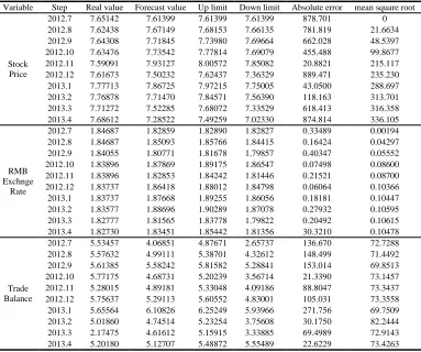
Table 1 Forecasting results in sample

Variable Step Real value Forecast value Up limit Down limit Absolute error mean square root

Stock Price

2012.7 7.65142 7.61399 7.61399 7.61399 878.701 0 2012.8 7.62438 7.67149 7.68153 7.66135 781.819 21.6634 2012.9 7.64308 7.71845 7.73980 7.69664 662.028 48.5397 2012.10 7.63476 7.73542 7.77814 7.69079 455.488 99.8677 2012.11 7.59091 7.93127 8.00572 7.85082 20.8821 215.117 2012.12 7.61673 7.50232 7.62437 7.36329 889.471 235.230 2013.1 7.77713 7.86725 7.97215 7.75005 43.0500 288.697 2013.2 7.76878 7.71470 7.84571 7.56390 118.163 313.701 2013.3 7.71272 7.52285 7.68072 7.33529 618.413 316.358 2013.4 7.68612 7.28522 7.49259 7.02330 874.814 336.105

RMB Exchnge

Rate

2012.7 1.84687 1.82859 1.82890 1.82827 0.33489 0.00194 2012.8 1.84687 1.85093 1.85766 1.84415 0.16424 0.04297 2012.9 1.84055 1.80771 1.81678 1.79857 0.40347 0.05552 2012.10 1.83896 1.87869 1.89175 1.86547 0.07498 0.08600 2012.11 1.83896 1.82853 1.84242 1.81446 0.21521 0.08700 2012.12 1.83737 1.86418 1.88012 1.84798 0.06064 0.10366 2013.1 1.83737 1.87668 1.89255 1.86056 0.18181 0.10447 2013.2 1.83577 1.88696 1.90289 1.87078 0.27932 0.10595 2013.3 1.82777 1.81565 1.83778 1.79822 0.20492 0.10615 2013.4 1.82730 1.83451 1.85442 1.81356 30.3210 0.10478

Trade Balance

2012.7 5.53457 4.06851 4.87671 2.65737 136.670 72.7288 2012.8 5.57632 4.99111 5.38701 4.32612 148.499 71.4492 2012.9 5.61385 5.58242 5.81582 5.28841 153.014 69.8513 2012.10 5.77175 4.68731 5.20239 3.56714 21.3390 73.1457 2012.11 5.28015 4.89181 5.33048 4.09186 88.8047 73.3437 2012.12 5.75637 5.29113 5.60552 4.83001 105.031 73.3558 2013.1 5.65564 6.10826 6.25249 5.93966 271.756 69.7509 2013.2 5.01860 4.74514 5.23254 3.75608 30.1750 82.2444 2013.3 2.17475 4.61612 5.15915 3.33885 69.4989 72.9143 2013.4 5.20180 5.12707 5.48872 5.55489 22.6229 73.4263

Fig.1 shows the real value and forecasting value of stock market price, the RMB exchange rate and the trade balance from July 2012 to April 2013. Thickened black line changes in the graphs represent the prediction results at different time points. The two dotted lines upper and lower is obtained through the prediction results which add and subtract RMS error t at different time point respectively, and then they form an error band. If the actual value falls into the standard error band in any unilateral side, , it is considered that this prediction is accurate.

(5)

[image:5.595.78.533.63.178.2]

(1) stock price (2) RMB real exchange rate (3)trade balance

Fig 1 Real value of three varibles and their forecasts

3. Impulse response analysis

In the VAR system, all variables are treated as endogenous variables which are symmetrically into various estimated equation, and can avoid the problems of omitted variables. Because the economic meaning obtained from the test results is difficult to analyze directly using the VAR model, it is often using impulse response function (Impulse Response Function, IRF) to analyses[10]. Impulse response analysis reflected that adding one impulse in the disturbance shows the impact on the current value and future value of endogenous variable. Koop et al (1996) presented improved response function method (Generalized Impulse Response Function, GIRF) to carry on the analysis, the decomposition of the does not rely on sequential relationship of the all variables in a VAR system, which improves the stability and reliability of the estimation results. This paper investigates one standard deviation of return on equity, RMB real exchange rate and the consumer impact on the current account and the dynamic impact Using this the impulse response function.

3.1Choice of variables and Data

As for variable selection, this paper mainly analyses three variables about Exchange rate, stock prices and the current account balance based on above Bayesian estimates. In the following analysis, in order to enhance the robustness of the test, this paper surveys with two variables about the consumer price index (CPI), the level of consumption (CONSUM) , and further investigate impact of the wealth effect of the financial market on current account. The data is from the July of 2005 to December of 2013. All variables are using monthly data. The data of real effective exchange rate of RMB (REER) is from the Bank for International Settlements, other relative data is from the National Bureau of Statistics. In order to reducing heteroscedasticity, all data were log processing.

3.2 Impulse response analysis

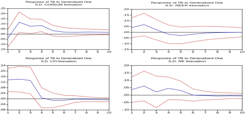
The testing results of impulse response function strongly depend on of the hypothesis that the error vector satisfies the white noise sequence vector, we first do stationary test for time series variables, and then through the different variables, such as the real exchange rate, return on equity, the level of consumption, the price level, this paper imposes a standard error on trade balance, and after that, investigates its different impulse response.

-.15 -.10 -.05 .00 .05 .10 .15 .20 .25

1 2 3 4 5 6 7 8 9 10 Response of TB to Generalized One

S.D. CONSUM Innovation

-.15 -.10 -.05 .00 .05 .10 .15 .20

S.D. REER Innovation

-.08 -.04 .00 .04 .08 .12 .16 .20 .24

S.D. CPI Innovation

-.10 -.05 .00 .05 .10 .15 .20

S.D. RE Innovation

Fig 2 Impulse response of Trade of Balance

[image:5.595.110.506.516.710.2]

(6)

maximum value in the second period. In the 2-6 period will emerge strong or weak small fluctuation, at last, after sixth period, the reaction is stable and close to 0. Second, there is a positive response for the shocks from the real effective exchange rate in 1-3 period, After the third period it gradually turn to negative response. And till the seventh period the reaction is close to 0. It can be seen that the impact of real effective exchange rate fluctuations on trade balance is more complex, which In different periods there have different effects. But in general, positive reaction is greater than the negative one, the positive reaction is up to the maximum in the second period.The trade balance response for the impact from inflation rate and stock returns are basically showing positive. The reaction to the inflation rate is experienced larger, persistent positive until 3rd period and then decreased rapidly to near 0. However, the response to equity return rate has a fluctuation change until the sixth period it is reduced to 0. In contrast, the trade balance response to each variable impact, such as consumption and inflate rate, show apparently larger, than those such as real effective exchange rate and stock price. The largest positive reaction of the real effective exchange rate and stock price is equal.

CONCLUSION

This paper theoretically analyses conduction pathway of exchange rate and stock price and the current account. First, using the Bayesian estimation method to predict the trade balance, the stock price and RMB exchange rate, it was concluded that there exists a certain relationship among the three variables , and forecasting the trend of the trade balance and the stock price is very accurate, the prediction of exchange rate is relatively low. In the subsequent analysis of pulse response, the consumption and the inflation rate of two intermediate variables are introduced in the paper. And we find that consumption have the more larger role the formation of Trade balance surplus of China than other factors such as RMB exchange rate and stock price. The effect of exchange rate to the trade balance are hysteretic.While the stock market on the trade balance surplus contribution is not obvious.

REFERENCES

[1] Zhu Mengnan, Liu.Lin. Financial Economy，2010(5):38-46

[2] Dong Ting. Journal of Zhejiang Industrial and Commercial University, 2010（01）：110-118．

[3] Zhao Wenjun. Study on World Economy,2010(1):3-11

[4] Cao Hui, Wang Wensheng. Journal of Economical Sdudy,2008（9）：56-58

[5] Wang Junbin, Guo Xinqiang. Financial Study, ,2011(11):47-61

[6] Chen Chuanglian. Journal of Shanxi Economic University,2013（9）:31-40

[7] Marcel Fratzscher. 2011, International Finance Discussion Paper.12:20-80. [8] Zhao Jinwen, Zhang jiangsi. Financial Study,2013（1）:9-23