Bootstrap based model selection in subset polynomial regression

87

Bootstrap-based model selection in subset polynomial

regression

Suparman a,1,*_{, Mohd Saifullah Rusiman} b,2

a _{Universitas Ahmad Dahlan, Yogyakarta, Indonesia} b _{Universiti Tun Hussein Onn Malaysia, Pagoh, Malaysia} 1_{[email protected] *;} 2 _{[email protected]} * corresponding author

1.

Introduction

The subset polynomial regression model is a polynomial regression in which some regression coefficients have a zero value. The advantage of this model is the user can select a regression model from all possible subsets of the polynomial regression model. The model has been studied by several researchers. Jekabson and Lavendels [1] compared the formation of polynomial regression models using the subset selection approach and the adaptive basis function construction approach. In the subset selection approach, the least squares method is used to approximate the solution. Overall the adaptive basis function construction approach was found to be superior to the subset selection approach. O'Neill et al. [2] used the method of a subset polynomial neural network to predict breast cancer. This method gives better results than the mammography method. Xie et al. [3] used the polynomial regression in medical image segmentation. Suparman [4] proposed a subset polynomial regression model using error which has an exponential distribution. The Markov Chain Monte Carlo (MCMC) reversible jump method is used to estimate the parameters of the subset polynomial regression model. The subset polynomial regression model often assumes that the error has a normal distribution or exponential distribution. However, in everyday life it is often found that the error distribution is unknown.

The Bootstrap method developed by Efroan and Tibshirani [5] is widely used in statistics and can be very useful in the context of regression [6]. A principle of the Bootstrap method is to try to get a good estimate based on minimal resources. In the case of statistical inference, minimal resources can be interpreted as small data, data that deviate from certain assumptions, and data that have no assumption about the distribution. Warton [6] used the bootstrap algorithm to estimate the parameters of a regression model. The Bootstrap method is applied in ecology. Garcia-Soidan et al. [7] used the Bootstrap method for spatial data. The estimator of the multivariate distribution function is used as the basis for the implementation of the Bootstrap method. Yazici et al. [8] used the Bootstrap method to obtain the empirical distribution of the parameters in the nonparametric regression of Conic Multivariate

A R T I C L E I N F O A B S T R A C T

Article history

Received April 6, 2018 Revised June 25, 2018 Accepted June 28, 2018

The subset polynomial regression model is wider than the polynomial regression model. This study proposes an estimate of the parameters of the subset polynomial regression model with unknown error and distribution. The Bootstrap method is used to estimate the parameters of the subset polynomial regression model. Simulated data is used to test the performance of the Bootstrap method. The test results show that the bootstrap method can estimate well the parameters of the subset polynomial regression model.

This is an open access article under the CC–BY-SA license.

Keywords

accurate parameter estimate. Beda et al. [9] used the Bootstrap method to calculate the confidence limits for spectral indices of heart-rate variability (HRV). Spectral indices are modeled using an autoregressive model. Hall and Maiti [10] used the Bootstrap method to construct a mean error estimator and to calculate the predicted region. The Bootstrap technique can be applied to non-normal models. Colugnati et al. [11] used the Bootstrap method to obtain interval estimation for percentiles on the diagnosis of obesity and overweight in children and adolescents. Kant et al. [12] used a bootstrap-based neural network model for flood estimates. The results show that the bootstrap-based neural network model is a stable model. Ren et al. [13] used the Bootstrap method to determine the confidence interval for multihop distances. The use of Bootstrap method can eliminate the risk of small sample size and unknown distribution. Kleiner et al. [14] used Bootstrap for massive data. Jacek et al. [15] used the Bootstrap approach to estimate the uncertainty of surface response models. Chen et al. [16] used a bootstrap analysis to measure individual and regional differences in relative concentrations of gamma-aminobutyric acid in the human brain. Dongping [17] used the Bootstrap method to determine predictive point and prediction intervals to reduce the risk of misleading decisions in maintenance in prognostic devices. Liang et al. [18] used the Bootstrap Metropolis-Hasting algorithm for model selection and optimization. Mei et al. [19] used the Residual-Based Bootstrap Test to detect the constant coefficients in the Weighted Geographic Regression model. Mikshowsky et al. [20] used bootstrap aggregation sampling to improve the reliability of genomic predictions for Jersey sires. Olaniran et al.

[21] used Bootstrap techniques to improve the selection and classification of Bayesian features. Zhen

[22] used Bootstrap resampling to detect wideband signal numbers. Boubaka et al. [23] used the Bootstrap method to identify parameters for the dependent data. In this paper, the Bootstrap method will be used to determine the parameter estimator in the polynomial subset regression. This paper aims to estimate the parameters of the subset polynomial regression model using the Bootstrap method.

2.

Method

The method used to estimate the parameters of the subset polynomial regression model is as follows:

2.1.The Least Squares Estimate

Suppose that (yt , xt) is the pairing of the dependent variable and the independent variable, as well as zt is error and t = 1, 2, ....n where n is the number of observation. Let kmax be a maximum order. The subset polynomial regression model which has an order k (k = 0, 1, ...., kmax) can be written as:

𝑦𝑡= 𝛽0+ 𝛽𝑛1𝑋𝑡 𝑛₁

+ 𝛽𝑛2𝑋𝑡 𝑛₂

+ ⋯ + 𝛽𝑛_𝑘𝑋𝑡 𝑛𝑘_{+ 𝑍}

𝑡  

Here {n1, n2, ..., nk} is the subset of {1, 2, ..., k} and 𝛽 = (𝛽₀, 𝛽_𝑛1, … , 𝛽_𝑛𝑘)′is the coefficient vector. The z_t (t = 1, 2, 3, ..., n ) is an error with mean 0 and variance 𝜎2 that is identical but its distribution is unknown. Based on the data (yt, xt) for t = 1, 2, ..., n, the parameters 𝛽, 𝜎2 and the polynomial regression subset models are estimated.

Equation (1) is a short form for a set of the following n simultaneous equations:

𝑦1= 𝛽0+ 𝛽𝑛1𝑋1 𝑛1_{+ 𝛽}

𝑛2𝑋1

𝑛2_{+ ⋯ + 𝛽}

𝑛𝑘𝑋1 𝑛𝑘_{+ 𝑍}

1  

𝑦2= 𝛽0+ 𝛽𝑛1𝑋2 𝑛1_{+ 𝛽}

𝑛2𝑋2

𝑛2_{+ ⋯ + 𝛽}

𝑛𝑘𝑋2 𝑛𝑘_{+ 𝑍}

2  



...

  

𝑦𝑛= 𝛽0+ 𝛽𝑛₁𝑋𝑛 𝑛₁

+ 𝛽𝑛₂𝑋𝑛 𝑛₂

+ ⋯ + 𝛽𝑛_𝑘𝑋𝑛 𝑛_𝑘

+ 𝑍𝑛  

In a matrix form, equation (2) can be written as:

where

𝑌 = [ 𝑌1

𝑌2

⋯ 𝑌𝑛

] , 𝑋 =

[

1 𝑋1

𝑛1

1 𝑋₂𝑛1

⋯ 1

⋯ 𝑋𝑛𝑛1

𝑋₁𝑛2 _{⋯ 𝑋}

1 𝑛𝑘

𝑋₂𝑛2 _{⋯ 𝑋}

2 𝑛𝑘

⋯ 𝑋_𝑛𝑛2

⋯ ⋯ 𝑋_𝑛𝑛𝑘

] , 𝛽 = [

𝛽0

𝛽𝑛1

⋯ 𝛽𝑛𝑘

] , 𝑎𝑛𝑑 𝑍 = [ 𝑍1

𝑍2

⋯ 𝑍𝑛

].

To obtain the least squares estimate of β, first write the sample subset polynomial regression:

𝑦𝑡= 𝛽̂0+ 𝛽̂𝑛1𝑋𝑡 𝑛₁

+ 𝛽̂𝑛2𝑋𝑡 𝑛₂

+ ⋯ + 𝛽̂𝑛_𝑘𝑋𝑡 𝑛𝑘_{+ 𝑍}

𝑡  

for t = 1, 2, 3, ..., n, which can be written briefly in matrix notation as:

𝑌 = 𝑋𝛽̂ + 𝑒  

where

𝑌 = [ 𝑌1

𝑌2

⋯ 𝑌𝑛

] , 𝑋 =

[

1 𝑋1

𝑛1

1 𝑋₂𝑛1

⋯ 1

⋯ 𝑋_𝑛𝑛1

𝑋₁𝑛2 _{⋯ 𝑋}

1 𝑛_𝑘

𝑋₂𝑛2 _{⋯ 𝑋}

2 𝑛_𝑘

⋯ 𝑋_𝑛𝑛2

⋯ ⋯ 𝑋_𝑛𝑛𝑘_]

, 𝛽̂ =

[ 𝛽̂0

𝛽̂𝑛₁

⋯ 𝛽̂𝑛_𝑘]

, 𝑎𝑛𝑑 𝑒 = [ 𝑒1

𝑒2

⋯ 𝑒𝑛

].

Here, 𝛽̂ is a column vector of the least squares estimator of the subset polynomial regression coefficient and e is a column vector of the residual n. According to the least squares method, the least squares estimator is obtained by minimizing (6).

∑𝑛𝑡=1𝑒𝑡2= ∑ (𝑦𝑡− 𝛽̂0− 𝛽̂𝑛1𝑋𝑡

𝑛1_{− ⋯ − 𝛽̂}

𝑛𝑘𝑋𝑡 𝑛_𝑘

)2

𝑛

𝑡=1   

This is achieved by partially differentiating (6) to 𝛽0, 𝛽𝑛₁, … , 𝛽𝑛_𝑘 and the result obtained is equal to

zero. This process produces k + 1 simultaneous equations in k + 1 unknown variables.

𝑛𝛽̂0+ 𝛽̂𝑛1∑ 𝑋𝑡 𝑛1

𝑛

𝑡=1 + 𝛽̂𝑛2∑ 𝑋𝑡 𝑛2

𝑛

𝑡=1 + ⋯ + 𝛽̂𝑛𝑘∑ 𝑋𝑡 𝑛𝑘

𝑛

𝑡=1 = ∑𝑛𝑡=1𝑦𝑡 

𝛽̂0∑ 𝑋𝑡 𝑛1

𝑛

𝑡=1 + 𝛽̂𝑛₁∑ 𝑋𝑡 2𝑛1

𝑛

𝑡=1 + 𝛽̂𝑛₂∑ 𝑋𝑡 𝑛1_𝑋

𝑡 𝑛2

𝑛

𝑡=1 + ⋯ + 𝛽̂𝑛_𝑘∑ 𝑋𝑡 𝑛1_𝑋

𝑡 𝑛_𝑘 𝑛

𝑡=1 = ∑ 𝑋𝑡

𝑛1_𝑦

𝑡 𝑛

𝑡=1  

𝛽̂0∑ 𝑋𝑡 𝑛2

𝑛

𝑡=1 + 𝛽̂𝑛1∑ 𝑋𝑡 𝑛2_𝑋

𝑡 𝑛1

𝑛

𝑡=1 + 𝛽̂𝑛2∑ 𝑋𝑡 2𝑛2

𝑛

𝑡=1 + ⋯ + 𝛽̂𝑛𝑘∑ 𝑋𝑡 𝑛2_𝑋

𝑡 𝑛𝑘

𝑛

𝑡=1 = ∑ 𝑋𝑡

𝑛2_𝑦

𝑡 𝑛

𝑡=1  

  

𝛽̂0∑ 𝑋𝑡 𝑛𝑘

𝑛

𝑡=1 + 𝛽̂𝑛1∑ 𝑋𝑡 𝑛𝑘_𝑋

𝑡 𝑛₁ 𝑛

𝑡=1 + 𝛽̂𝑛2∑ 𝑋𝑡 𝑛𝑘_𝑋

𝑡 𝑛₂ 𝑛

𝑡=1 + ⋯ + 𝛽̂𝑛_𝑘∑ 𝑋𝑡 2𝑛𝑘

𝑛

𝑡=1 = ∑ 𝑋𝑡

𝑛𝑘_𝑦

𝑡 𝑛

𝑡=1  

In the matrix form, equation (7) can be presented as:

(𝑋′_{𝑋)𝛽̂ = 𝑋}′_{𝑌  }

If the inverse of (X'X) exists, say (X'X)-1_{, then by multiplying in both sides of (8) by this inverse, the} result is as follows:

(𝑋′_𝑋)−1_(𝑋′_{𝑋)𝛽̂ = (𝑋}′_𝑋)−1_𝑋′_{𝑌  }

or

𝛽̂ = (𝑋′𝑋)−1𝑋′𝑌  

The least squares estimator for 𝛽 = (𝛽0, 𝛽𝑛1, … , 𝛽𝑛𝑘) ′ _is

and the least squares estimator for 𝜎2 is:

𝜎̂2₌𝑌′𝑌−𝛽̂′𝑋′𝑌

𝑛−𝑘−1   

2.2.Statistical Criteria

The Ck statistical criteria [5] is used to select the best polynomial subset regression model. The best subset polynomial regression model selected is a subset polynomial regression model that has the smallest Ck value. The Ck value is calculated using the following equation:

𝐶𝑘 =

∑𝑛𝑡=1(𝑦𝑡 − 𝛽̂0 − 𝛽̂𝑛1𝑋𝑡𝑛1− ⋯− 𝛽̂𝑛𝑘𝑋𝑡𝑛𝑘)2

𝑛 −

2𝑘𝜎̂2

𝑛   

2.3.Bootstrap Method

The Bootstrap method developed in [5] is a simulation method based on data that can be applied to statistical inference problems. A basic principle of bootstrapping is resampling i.e. resampling / artificial observation of z1, z2, ... , zn that already exists.

F

ˆ

is an empirical distribution taken with probability 1/n at each observed value z1, z2, ..., zn. Let B be a number of the resampling. The Bootstrap sample is defined as a random sample of size n composed of

F

ˆ

, e.g. the bth _{Bootstrap sample (b = 1, 2, ... , B) is denoted by} b

n b 2 b

1,z ,...,z

z . The Bootstrap sample

b n b 2 b

1,z ,...,z

z is a random sample of size n taken with the return of population z1, z2, ..., zn. Members

of the bootstrap sample b

n b 2 b

1,z ,...,z

z comprising the original samples z1, z2, ..., zn, appear once, appear twice, appear more than twice, or do not appear in the original sampling process. The computational steps to determine the 100(1-α)% confidence interval for 𝑦̂𝑡+1 are as follows:

1) Calculate 𝛽̂ and 𝜎̂2 _{from the original data.}

2) Calculate 𝑧̂𝑡 using the equation

𝑧̂𝑡= 𝑦̂𝑡− 𝛽̂0− 𝛽̂𝑛1𝑋𝑡

𝑛1_{− ⋯ − 𝛽̂}

𝑛𝑘𝑋𝑡

𝑛𝑘_{  }

3) For b = 1, 2, ...., B:

a. Resampling 𝑧̂_𝑡(𝑏).

b. Compute 𝑦̂_𝑡(𝑏) with the equation

𝑦̂_𝑡(𝑏)= 𝛽0+ 𝛽𝑛1𝑋𝑡

𝑛1_{+ ⋯ + 𝛽}

𝑛𝑘𝑋𝑡 𝑛𝑘_{+ 𝑧̂}

𝑡

(𝑏)_{  }

c. Compute 𝛽̂(𝑏), 𝜎̂2(𝑏), and 𝑦̂_𝑡+1(𝑏).

4) Compute 𝛽̂𝑏𝑜𝑜𝑡, 𝜎̂𝑏𝑜𝑜𝑡2 , and 𝑦̂(𝑡+1)(𝑏𝑜𝑜𝑡) (𝑏)

.

5) Calculate the 100(1-α)% confidence interval for 𝑦̂𝑡+1

3.

Results and Discussion

3.1. Simulated Data

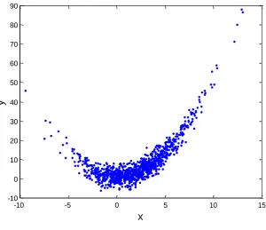
[image:5.595.156.457.135.394.2]

Fig. 1 shows a graph of 1000 synthesis data of the subset polynomial regression model with order 2. The value of x is determined, hence the value of y is made using equation (1). The values of regression coefficients and the variance of error are 𝛽0= 1, 𝛽2= 0.5, and 𝜎2=9.

Fig. 1.Simulated data

The simulated data in Fig. 1 are matched against the subset polynomial regression model i.e. kmax = 2. The Bootstrap algorithm is used to estimate the best subset polynomial regression model, the subset polynomial regression coefficient and the variance 𝜎2. Estimation of the subset polynomial regression model is done by looking at 𝐶𝑘 statistical value for the three regression models of the subset polynomial.

[image:5.595.182.429.517.597.2]

The 𝐶𝑘 statistical value for the three regression models of the subset polynomial can be seen in Table 1.

Table 1. The Ck statistical value Subset Polynomial Regression

Model with Order 2

Ck Statistical Value

𝑦 = 𝛽0+ 𝛽1𝑋 62.5997

𝑦 = 𝛽0+ 𝛽2𝑋2 9.1938

𝑦 = 𝛽0+ 𝛽1𝑋 + 𝛽2𝑋2 9.2170

From Table 1 it can be seen that the smallest 𝐶𝑘 statistical value is achieved by the second subset

polynomial regression model. Thus, the second regression is the best subset polynomial regression model. Based on the regression of the best subset polynomial, then the parameters of the corresponding subset polynomial regression model are estimated using the least squares method. The results are 𝛽̂0=

0.9323, 𝛽̂2= 0.5070, and 𝜎̂2= 9.1756. If the parameter values and estimator values of both regression

and variance coefficients are compared then it appears that the Bootstrap algorithm can work well in estimating parameters based on synthesis data. Prediction for the value of y1000 if x = 16.4176 is 9.2569 and the corresponding 95% confidence interval is (9.0984, 9.4117).

3.2. Real Data

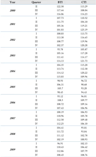
Table 2 shows the business tendency index (y) and the consumer tendency index (x) in the second

-10 -5 0 5 10 15

-10 0 10 20 30 40 50 60 70 80 90

x

[image:6.595.141.467.103.637.2]

Table 2. The business tendency index (BTI) and the consumer tendency index (CTI)

Year Quarter BTI CTI

2000

II 122.50 113.29

III 117.44 108.04

IV 116.06 114.23

2001

I 107.73 110.52

II 111.75 104.10

III 105.36 119.21

IV 101.03 125.19

2002

I 100.03 113.75

II 113.38 116.65

III 108.77 119.96

IV 102.37 120.28

2003

I 95.78 105.87

II 105.16 117.28

III 111.41 114.17

IV 114.13 121.73

2004

I 104.35 115.20

II 113.74 112.30

III 114.12 120.22

IV 115.03 109.96

2005

I 98.93 96.72

II 106.31 98.68

III 105.7 93.20

IV 98.45 94.43

2006

I 95.12 96.01

II 108.5 109.77

III 108.72 109.16

IV 107.43 106.96

2007

I 100.19 106.93

II 110.96 105.78

III 112.58 109.48

IV 112.25 106.10

2008

I 104.41 95.01

II 111.72 93.84

III 111.12 102.78

IV 102.19 100.93

2009

I 96.91 102.15

II 110.43 106.42

III 112.86 107.79

IV 108.45 108.76

Source: http://www.bps.go.id

The data in Table 2 are matched against the subset polynomial regression model. Here kmax = 3. The bootstrap algorithm was used to obtain the subset polynomial regression model, the regression model parameters, and the variance 𝜎2_{. Estimation of subset polynomial regression model is done by looking}

at the statistical value of 𝐶𝑘 for 7 models.

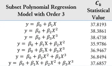
From Table 3 it can be seen that the smallest 𝐶𝑘 statistical value is achieved by the 4th subset

[image:7.595.209.402.91.206.2]

Table 3. The Ck statistical value Subset Polynomial Regression

Model with Order 3

𝑪𝒌

Statistical Value

𝑦 = 𝛽0+ 𝛽1𝑋 37.8193

𝑦 = 𝛽0+ 𝛽2𝑋2 38.3861

𝑦 = 𝛽0+ 𝛽3𝑋3 38.4738

𝑦 = 𝛽0+ 𝛽1X + 𝛽2𝑋2 35.9786

y = 𝛽0+ 𝛽1X + 𝛽3𝑋3 36.9467

y = 𝛽0+ 𝛽2𝑋2+ 𝛽3𝑋3 36.8494

y = 𝛽0+ 𝛽1X + 𝛽2𝑋2+ 𝛽3𝑋3 37.6857

Based on this subset best polynomial regression model, then the parameters of the corresponding subset polynomial model are estimated. The results are 𝛽̂0= −189.1774, 𝛽̂1= 5.2858, 𝛽̂2= −0.0234,

and 𝜎̂2_{= 32.6954. The prediction for y}

41 if x = 108.76 is 108.7878 and the 95% confidence interval for y41 if x = 108.76 is (106.8255, 110.7612).

4.

Conclusion

The paper showed how the Bootstrap algorithm can be used to generate parameter estimations in the polynomial subset regression model and determine the prediction interval for the dependent variable in the polynomial subset regression model if the error has any distribution. The simulation results showed that the Bootstrap algorithm could estimate well the parameters and determine the prediction interval. The obtained subset polynomial regression model would be very useful for decision making, for example, to predict the value or calculate the prediction interval of variable y in the future.

Acknowledgment

The authors would like to thank Assoc. Prof. Allan Leslie White, Ph.D., University of Western Sydney, for his suggestions to improve this paper.

References

[1] G. Jekabsons and J. Lavendels, “A Comparison of Subset Selection and Adaptive Basis Function Construction for Polynomial Regression Model Building,” Computer Sciences, vol. 38, no. 38, pp. 187-197, 2009, doi: https://doi.org/10.2478/v10143-009-0017-7.

[2] T. O’Neill, J.Penm and J.S. Penm, “A Subset Polynomial Neural Networks Approach for Breast Cancer Diagnosis,” International Journal of Electronic Healtheare, vol. 3, no. 3, pp. 293-302. 2007, doi: https://doi.org/10.1504/IJEH.2007.014549.

[3] C.H. Xie, Y.J. Liu and J.Y. Chang, “Medical Image Segmentation Using Rough Set and Local Polynomial Regression,” Multimedia Tools and Applications, vol. 74, no. 6, pp. 1885-1914, 2015, doi: https://doi.org/ 10.1007/s11042-013-1723-2.

[4] Suparman, “Selection in Subset Polynomial Regression by Using Reversible Jump MCMC,” Journal of

Environmetal Science, Computer Science and Engineering & Technology, vol. 5, no. 3, pp. 214-219, 2016,

available at: http://eprints.uad.ac.id/3374/1/JecetVol5No3Thn2016.pdf.

[5] B. Efron and R. Tibshirani, An Introduction to the Bootstrap. Chapman & Hall : New York, 1993, doi: https://doi.org/10.1007/978-1-4899-4541-9.

[6] D. Warton, L. Thibaut and Y.A. Wang, “The PIT-trap-A “model-tree” Bootstrap Procedure for Inference about Regression Models with Discrete,” Multivariate Responses, PloS ONE, vol. 12, no. 7, pp. 1-18, 2017, doi: https://doi.org/10.1371/journal.pone.0181790.

[7] P. Carcia-Soidan, R. Menezes and O. Rubinos, “Bootstrap Approaches for Spatial Data,” Stochastic

Environmental Research & Risk Assessment, vol. 28, no. 5, pp. 1207-1219, 2014, doi: https://doi.org/

[8] C. Yazici, I. Batnaz and F. Yerlikaya-Ozkurt, “A Computational Approach to Nonparametric Regression : Bootstrapping CMARS Method,” Machine Learning, vol. 101, no. 1, pp. 211-230, 2015, doi: https://doi.org/10.1007/s10994-015-5502-3.

[9] A. Beda, D.M. Simpson and L. Faes, “Estimation of Confidence Limits for Descriptive Indexes Derived from Autoregressive Analysis of Time Series : Methods and Application to Heart Rate Variability,” PLoS

ONE, vol. 12, no. 10, pp. 1-22, 2017, doi: https://doi.org/10.1371/journal.pone.0183230.

[10]P. Hall and T. Maiti, “On Parametric Bootstrap Methods for Small Area Prediction,” Journal of the Royal

Statistical Society : Series B, vol. 68, no. 2, pp. 221-238, 2006, doi:

https://doi.org/10.1111/j.1467-9868.2006.00541.x.

[11]F.A.B Colugnati, F. Louzada-Neto and J.A. Taddei, “An Application of Bootstrap Resampling Method to Obtain Confidence Interval for Percentile Fatness Cutoff Points in Childhood and Adolescence Overweight Diagnoses,” International Journal of Obesity, vol. 29, no. 3, pp. 340-347, 2005, doi: https://doi.org/ 10.1038/sj.ijo.0802866.

[12]A. Kant, P.K. Suman, B.K. Giri, M.K. Tiwari, C. Chatterjee, P.C. Nayak and S. Kumar, “Comparison of Multi-Objective Evolutionary Neural Network, Adaptive Neuro-Fuzzy Inference System and Bootstrap-Based Neural Network for Flood Forecasting,” Neural Comput & Applic, vol. 23, no. 1, pp. 231-246, 2013, doi: https://doi.org/10.1007/s00521-013-1344-8.

[13]Y. Ren, N. Yu, X. Wang, L. Li and J. Wan, “Nonparametric Bootstrap-Based Multihop Localization Algorithm for Large-Scale Wireless Sensor Networks in Complex Environments,” International Journal of

Distributed Sensor Networks, pp. 1-9, 2013, doi: https://doi.org/10.1155/2013/923426.

[14]A. Kleiner, A. Talwalkar, P. Sarkar and M.I. Jordan, “A Scalable Bootstrap for Massive Data,” J.R. Statist.

Soc. B, vol. 76, no. 4, pp. 795-816, 2014, doi: https://doi.org/10.1111/rssb.12050.

[15]P. Jacek, R. Norbert, S. Malgorzata, G. Andrii and K. Maciej, “Bootstrap Identification of Confidence Intervals for the Non-Linear DoE Model,” Applied Mechanics and Materials, vol. 712, pp. 11-16, 2015, doi: https://doi.org/10.4028/www.scientific.net/AMM.712.11.

[16]M. Chen, C, Liao, S. Chen, Q. Ding, D. Zhu, H. Liu X. Yan and J. Zhong, “Uncertainty Assessment of Gamma-Aminobutyric Acid Concentration of Different Brain Regions in Individual and Group Using Residual Bootstrap Analysis,” Med Biol Eng Comput, vol. 55, pp. 1051-1059, 2017, doi: https://doi.org/10.1007/s11517-016-1579-5.

[17]L. Dongping, “Failure Prognosis with Uncertain Estimation Based on Recursive Models Re-Sampling Bootstrap and ANFIS,” IAENG International Journal of Computer Science, vol. 43, no. 2, pp. 253-262, 2016, available at: http://www.iaeng.org/IJCS/issues_v43/issue_2/IJCS_43_2_15.pdf.

[18]F. Liang, J. Kim and Q. Song, “A Bootstrap Metropolis-Hastings Algorithm for Bayesian Analysis of Big Data,” Technometrics, vol. 58, no. 3, pp. 304-318, 2016, doi: https://doi.org/10.1080/00401706.2016.1142905. [19]C-L Mei, M. Xu and N. Wang, “A Bootstrap Test for Constant Coefficients in Geographically Weighted Regression Models,” International Journal of Geographical Information Science, vol. 30, no. 8, pp. 1622-1643, 2016, doi: https://doi.org/10.1080/13658816.2016.1149181.

[20]A.A. Mikshowsky, D. Gianola and K.A. Weigel, “Improving Reliability of Genomic Predictions for Jersey Sires Using Bootstrap Aggregation Sampling,” J. Dairy Sci., vol. 99, pp. 3632-3645, 2016, doi: https://doi.org/10.3168/jds.2015-10715.

[21]O.R. Olaniran, S.F. Olaniran, W.B. Yahya, A.W. Banjoko, M.K. Garba, L.B. Amusa and N.F Gatta, “Improved Bayesian Feature Selection and Classification Methods Using Bootstrap Prior Techniques,” Anale.

Seria Informatica., vol. 14, no. 2, pp. 46-52, 2016, available at: http://anale-informatica.tibiscus.ro/download/

lucrari/14-2-07-Olaniran.pdf.

[22]J. Zhen, “Detection of Wideband Signal Number Based on Bootstrap Resampling,” International Journal of

Antennas and Propagation, pp. 1-8, 2016, doi: https://doi.org/10.1155/2016/3856727.

[23]T. Boukaba, M.N.E. Korso, A.M. Zoubir and D. Berkani, “Bootstrap Based Sequential Detection in Non-Gaussian Correlated Clutter,” Progress in Electromagnetics Research, vol. 81, pp. 125-140, 2018, doi: