International Journal of Emerging Technology and Advanced Engineering
Website: www.ijetae.com (ISSN 2250-2459, Volume 2, Issue 9, September 2012)503
A Technical Survey on Cluster Analysis in Data Mining.
Yaminee S. Patil
1,M.B.Vaidya
2,1AVCOE Sangamner, INDIA.
2AVCOE Sangamner, INDIA.
Abstract—In data mining functionalities, clustering analysis is the most significant tool for distribution of data. Clustering is dynamic field of research in data mining concept. It is related to unsupervised learning in machine learning. On the basis of similarity measures cluster formation process is initiated. With the help of different notations used in clustering algorithms unique clusters are formed with the same data set. In this paper several clustering methods are discussed with their particular algorithms. Clustering methods are drastically affecting the shapes of cluster, quality of cluster, scalability of clusters. In this paper we have discussed integrated clustering algorithm that is multiphase clustering algorithms which improves scalability and efficiency of clusters. Different algorithms perform different task to make cluster more dynamic and effective. Several clustering methods and their corresponding algorithms are described below which helps to further analysis.
Keywords— Clustering analysis, data mining, multiphase clustering, similarity measures, unsupervised learning.
I. INTRODUCTION
Data mining is truly interdisciplinary topic which can be defined in many different ways. In the field of database management industry data analysis is mainly evolved with number of large data repositories. The result yields to the process of data mining. There are a number of data mining functionalities are used to specify the kinds of patterns to be found in data mining task. These functionalities include characterizations and discrimination, the mining of frequent patterns, associations and correlations, classification and regression; clustering analysis, outlier analysis. In this paper we are providing a wide approach to clustering analysis.Clustering is one of the most interesting and important topics in data mining. The aim of clustering is to find intrinsic structures in data, and organize them into meaningful subgroups for further study and analysis. Clustering as a data mining tool has its root in many application area such as biology, image pattern recognition, security, business intelligence and Web search. Cluster analysis [2]can be used as a standalone data mining tool to achieve data distribution, or as a pre-processing step for other data mining algorithms operating on the detected clusters.
The basic concept of cluster analysis is the process of partitioning a set of data objects or observations into subset; each subset is unique clusters such that objects are in one cluster are similar to one another, yet dissimilar to objects in other cluster. Different cluster may be formed using same data set by applying different clustering methods. There are many well established clustering algorithm are present in literature. These can be categorized from several orthogonal aspects such as those regarding partitioning criteria, separations of clusters [1], similarity measures used and clustering space. In this paper we will discuss the major fundamental clustering methods [3] such as, partitioning methods, hierarchical methods, density-based methods and grid-density-based methods.
Partitioning method conducts one-level partitioning on data set, first it creates initial set of k partition, where parameter k is the number of partition to construct. It then uses an iterative relocation technique that attempts to improve the partitioning by moving objects from one group to another group. Typical partitioning method includes two popular algorithms, k-means [1][4], and k-medoids.
Hierarchical method creates a hierarchical decomposition of the given set of data objects. The hierarchical method [5] can be classified as being either agglomerative on how the hierarchical decomposition is formed. This method suffers from the fact that once step is done it can never be undone. This rigidity is useful in smaller computation. Now a day many algorithms are devised to improve the clustering quality of hierarchical method is to integrate with other clustering methods, resulting now we are introducing multiphase clustering. Typically multiphase clustering method includes two popular algorithm, BIRCH [6], and chameleon [7].
Density–based methods [8] are mostly use to find arbitrary shaped clusters in this clusters objects based on notation of density. It grows cluster either according to the density of neighbourhood objects or according to the density function. The popular algorithms are, DBSCAN, and OPTICS.
International Journal of Emerging Technology and Advanced Engineering
Website: www.ijetae.com (ISSN 2250-2459, Volume 2, Issue 9, September 2012)504 tendency, determining the number of cluster and measuring cluster quality. These points help us to determine the cluster efficiency and cluster scalability.
The remaining paper is organized as follows: In section 2, we review related literature on data mining and clustering analysis. It is followed by basic clustering methods in section 3. Section 4 contains clustering algorithms. Finally we are concluding in section 5.
II. LITERATURE ON DATA MINING CLUSTER ANALYSIS The field of data mining is multidisciplinary; it can be express by many different ways. Data mining (sometimes called knowledge discovery) is the process of analyzing data from different views and summarizing it into useful information this information is nothing but knowledge that can be used to increase revenue of information. Conceptually data mining is very essential step in knowledge discovery from variety of large data tombs. Data mining tools [10][3] process data to discover interesting patterns or knowledge. The data source includes database, data warehouse, the Web, other data repositories and the data which are streamed into the system dynamically. This data may be in various forms as quantitative, spatial, specific semantics, hypertext and multimedia, special structures. The richest information repositories are relational database which are used to study data mining. Technically, data mining is the process of finding correlations or patterns among dozens of fields in large relational databases. To recognize different patterns of knowledge we use similarity and dissimilarity measures. We measures object’s similarity and dissimilarity by comparing objects with each other in data mining methodologies such as clustering analysis, outlier analysis and nearest-neighbor classification. These measures include distance measures like Euclidean distance, Manhattan distance, supremum distances between two objects of numeric data. Data mining functionalities are mostly used to recognize the different patterns found in data mining task; generally these tasks are of two types: descriptive and predictive. Descriptive data mining task describe the properties of data in target data set and predictive data mining task formally introduce the current data in order to make predictions. Data mining is highly application driven domain.it incorporated many techniques from many domain such as statistics, machine learning, pattern reorganization, data warehouse system, information retrieval, visualization, algorithms, high performance computing, and many more application domains. As data mining adopts many techniques that strongly influence the development of data mining functionalities.
Data mining functionalities include clustering analysis; it can be used as a single tool for understanding distribution of data, to observe the characteristics of each cluster, and focus on clusters for further analysis. The basic concept of cluster analysis [2] or clustering is the process of partitioning large data set of objects into small subsets. Each small subset is a unique cluster, such that the objects are clustered together based on the principle of maximizing the intraclass similarity and minimizing interclass similarity. That is, clusters are so formed that objects within cluster have high similarity with other objects present in the same cluster, but are rather dissimilar to objects in other clusters. Similarity and dissimilarity are assessed based on the attribute values describing objects and different distance measures. The set of clusters resulting from clustering analysis of large data tombs can be referred as clustering. Clustering is nothing but the data segmentation because clustering partitions large data set into groups according to their similarity measure. It also used for outlier detection where in some cases outliers are more interesting than normal and usual cases. For clustering task machine learning research often focuses on the accuracy of the model. Unsupervised learning is proper synonym for clustering because class label information is not present. Therefore clustering analysis is a form of learning by observation rather than learning by examples. Therefore, clustering is unsupervised learning of a hidden data concept. Clustering [2] [3]is dynamic and challenging research field of data mining which focused on finding methods for effective and efficient cluster analysis in large database.
III. BASIC CLUSTERING METHODS
A. Partitioning Method
International Journal of Emerging Technology and Advanced Engineering
Website: www.ijetae.com (ISSN 2250-2459, Volume 2, Issue 9, September 2012)505 Most of the applications adopt popular heuristic methods such as greedy approaches like k-means [4] and k-medoids algorithms, which progressively improve the clustering quality. Mostly this heuristic method of clustering generates spherical shaped clusters in small-to-medium size database. To find different complex shaped cluster with large database, partitioning methods need to be extended.
B. Hierarchical Method
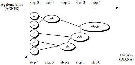
[image:3.612.54.279.479.588.2]Hierarchical method [5] creates hierarchical decomposition of the given data set of data objects. Representation of data objects into hierarchy is useful for data visualization and summarization in a compressed way. Hierarchical method is classified as being either agglomerative or divisive based on the decomposition is formed. Agglomerative method uses bottom-up strategy. It typically starts with each object to form its own cluster and iteratively merges clusters into larger and larger clusters, until all objects form a single cluster or some termination condition satisfied. For the merging step first we have to check the two clusters are closet to each other according to some similarity measure and then combine these two clusters to form a single cluster. Divisive method uses top-down strategy. It typically starts with all objects in a single cluster as a hierarchy root. It then divides root into several sub-clusters. It recursively partition the clusters until each cluster at the lowest level is a cluster with only single object or some termination condition is satisfied as shown in figure 1.
Fig 1: Agglomerative and divisive hierarchial clustering on data objects
In either agglomerative or divisive hierarchical clustering a user can specify the desired number of clusters as a termination condition. Hierarchical clustering method unexpectedly faces with the difficulties regarding the selection point of merge and split. This decision regarding with split and merge points is difficult because once we select the point then new cluster is formed according to selected point. The major drawback of hierarchical clustering, once a step (merge or split) is done, neither it
can be not undone nor perform object swapping in between clusters. To overcome this drawback we have a promising direction for improving hierarchical clustering method, is to integrate hierarchical clustering method with other clustering techniques resulting multiphase clustering. Multiphase clustering introduces two popular algorithms BIRCH [6] and chameleon begins by partitioning objects hierarchically using tree structures where leaf or non-leaf nodes can be viewed as micro-clusters. It then applies to other clustering algorithms to create macro-clustering on micro-clusters. Chameleon [7] explores dynamic modelling in hierarchical clustering.
C. Density based clustering method
Most of clustering methods like partitioning method or hierarchical method, clusters are based on distance between objects therefore they create spherical shaped clusters only. Density based clustering method [8] use notation density for formation of clusters. And with this density based clustering method can create clusters of arbitrary shape such as oval or s-shape. The general idea is to continue growing a given cluster as long as the density (number of objects or data points) in the neighbourhood exceeds some threshold. Density based clustering method divide a set of data objects into multiple exclusive clusters or in hierarchy of clusters, the popular algorithms are DBSCAN, and OPTICS.
D. Grid based clustering method
Grid based clustering approach uses a multiresolution grid structure. Grid based method takes a space driven approach by partitioning the embedded space into cells independent of the distribution of the input objects. The main advantage of this method is fast processing time which never gets affected by the number of objects, and the cells in dimensions in the quantized space. Two typical examples, STING [9] which explores statistical information stored in the grid cells and CLIQUE represents a grid and density based approach for subspace clustering in a high dimensional data space.
IV. ALGORITHMS
A. k-means
International Journal of Emerging Technology and Advanced Engineering
Website: www.ijetae.com (ISSN 2250-2459, Volume 2, Issue 9, September 2012)506 The difference between an object p ϵ Ci and ci, the representative of the cluster, is measured by dist (p, ci), where dist (x,y) is the Euclidean distance between two points x and y. the quality of cluster Ci, can be measured by the within cluster variation, which is the sum of squared error between all objects in Ci, and the centroid ci defined as,
𝐸 = 𝑑𝑖𝑠𝑡(𝑝, 𝑐
𝑖)
2 𝑝∈𝐶𝑖𝑘
𝑖=1
Where E is the sum of the squared error for all objects in the data set; p is the point in space representing a given object; and ci is the centroid of cluster Ci. In other words, for each object in each cluster, the distance from the objects to its cluster is squared, and the distances are summed. The objective function tries to make the resulting K-clusters as unique as possible. The K-means algorithm proceeds as follows:
Algorithm: K-means: the K-mean algorithm for
partitioning, where each cluster’s centre is represented by the mean value of the objects in the cluster.
Input: K: the number of clusters D: a data set containing n objects Output: A set of K cluster
Method:
1. Arbitrarily choose K objects from D as the initial cluster’s centers;
2. Repeat
3. (Re) assign each object to the cluster to which the object is most similar, based on the mean value of the objects in the cluster;
4. Update the cluster means, that is, calculate the mean value of the objects for each cluster;
5. Until no change
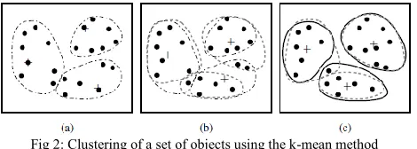
Example of K-mean: Consider a set of objects located in
[image:4.612.53.288.584.668.2]2-D space as shown in figure 2. Let K=3. In figure 2, the centers are marked by +, each object is assigned to a cluster based on the cluster centre to which it is nearest.
Fig 2: Clustering of a set of objects using the k-mean method
Each object is assigned to a cluster based on the center to which it is the nearest. Such a distribution forms silhouettes encircled by dotted curves, as shown in figure 2.
Next, the cluster centers are updated. That is, the mean value of each cluster is recalculated based on the current objects in the cluster. Using the new cluster centers, the objects are redistributed to the clusters based on which cluster center is the nearest. Such are distribution forms new silhouettes encircled by the dashed curves, as shown in the figure 2(b).
This process iterates, leading to figure 2(c). The process of iteratively reassigning objects to clusters to improve the partitioning is referred to as iterative relocation. Eventually, no reassignment of the objects in any cluster occurs and so the process terminates. The results may depend on the initial random selection of cluster centers. To obtain good results in practice, it is common to run the K-means algorithm multiple times with different initial cluster centers.
The time complexity of the k-means algorithm is O(nkt), where n is the total number of objects, k is the number of clusters, and t is the number of iterations. Normally, k<<n and t<<n. Therefore, the method is relatively scalable and efficient in processing large data sets.
B. K medoids
The k-means algorithm is sensitive to outliers because an object with an extremely large value may substantially distort the distribution of data. Instead of taking the mean value of the objects in a cluster as a reference point, we can pick actual objects to represent the clusters, using one representative object per cluster. Each remaining object is clustered with the representative object to which it is the most similar. The partitioning method is then performed based on the principle of minimizing the sum of the dissimilarities between each object and its corresponding reference point. That is, an absolute-error criterion is used, defined as
𝐸 = 𝑑𝑖𝑠𝑡(𝑝, 𝑜
𝑖)
𝑝∈𝐶𝑖 𝑘
𝑖=1
International Journal of Emerging Technology and Advanced Engineering
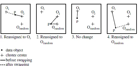
Website: www.ijetae.com (ISSN 2250-2459, Volume 2, Issue 9, September 2012) [image:5.612.52.287.133.246.2]507 Fig 3: Four cases of the cost function for k-medoids clustering
Case 1: p currently belongs to representative object, oj. If oj is replaced by orandom as a representative object and p is closest to one of the other representative objects, oi, i 6= j, then p is reassigned to oi.
Case 2: p currently belongs to representative object, oj. If
oj is replaced by orandom as a representative object and p is closest to orandom, then p is reassigned to orandom.
Case 3: p currently belongs to representative object, oi, i 6=
j. If oj is replaced by orandomas a representative object and p is still closest to oi, then the assignment does notchange. Case 4: p currently belongs to representative object, oi,i 6=
j. If ojis replaced by orandomas a representative object and p is closest to orandom, then p is reassigned to orandom.
Each time a reassignment occurs, a difference in absolute error, E, is contributed to the cost function. Therefore, the cost function calculates the difference in absolute-error value if a current representative object is replaced by a non-representative object. The total cost of swapping is the sum of costs incurred by all non-representative objects. If the total cost is negative, then oj is replaced or swapped with orandom since the actual absolute error E would be reduced. If the total cost is positive, the current representative object, oj, is considered acceptable, and nothing is changed in the iteration. PAM(Partitioning Around Medoids) was one of the first k-medoids algorithms introduced (Figure 3).The complexity of each iteration is O(k(n-k)2). For large values of n and k, such computation becomes very costly.
Algorithm: k-medoids. PAM, a k-medoids algorithm for
partitioning based on medoids or central objects. Input: k:the number of clusters,
D: a data set containing n objects. Output: A set of k clusters.
Method:
1. Arbitrarily choose k objects in D as the initial representative objects or seeds;
2. Repeat
3. Assign each remaining object to the cluster with the nearest representative object;
4. Randomly select a non-representative object, o random;
5. Compute the total cost, S, of swapping representative object, oj, with o random;
6. If S < 0 then swap oj with o random to form the new set of k representative objects;
7. Until no change;
A typical k-medoids partitioning algorithm like PAM works effectively for small data sets, but does not scale well for large data sets. To deal with larger data sets, a sampling-based method, called CLARA (Clustering Large Applications) [1], can be used. The effectiveness of CLARA depends on the sample size. Notice that PAM searches for the best k medoids among a given data set, whereas CLARA searches for the best k medoids among the selected sample of the data set. CLARA will never find the best clustering. A good clustering based on sampling will not necessarily represent a good clustering of the whole data set if the sample is biased.
C. BIRCH: Balance Iterative Reducing And Clustering
Using Hierarchies
BIRCH [1] [6] is designed for clustering a large amount of numerical data by integration of hierarchical clustering (at the initial micro-clustering stage) and other clustering methods such as iterative partitioning (at the later macro-clustering stage). It overcomes the two difficulties of agglomerative clustering methods: (1) scalability and (2) the inability to undo what was done in the previous step. BIRCH introduces two concepts, clustering feature and clustering feature tree (CF tree), which are used to summarize cluster representations. These structures help the clustering method achieve good speed and scalability in large databases and also make it effective for incremental and dynamic clustering of incoming objects. Given n d-dimensional data objects or points in a cluster, we can define the centroid x0, radius R, and diameter D of the cluster as follows:
𝑥
0=
𝑥
𝑖𝑛 𝑖=1
𝑛
=
𝐿𝑆
𝑛
𝑅 =
𝑥
𝑖− 𝑥
𝑜 2𝑛 𝑖=1
𝑛
=
𝑛𝑆𝑆 − 2𝐿𝑆
2+ 𝑛𝐿𝑆
𝑛
2𝐷 =
𝑥
𝑖− 𝑥
𝑗2 𝑛
𝑗 =1 𝑛 𝑖=1
𝑛(𝑛 − 1)
=
2𝑛𝑆𝑆 − 2𝐿𝑆
2International Journal of Emerging Technology and Advanced Engineering
Website: www.ijetae.com (ISSN 2250-2459, Volume 2, Issue 9, September 2012)508 where R is the average distance from member objects to the centroid, and D is the average pairwise distance within a cluster. Both R and D reflect the tightness of the cluster around the centroid. A clustering feature (CF) is a three-dimensional vector summarizing information about clusters of objects. Given n d-dimensional objects or points in a cluster, then the CF of the cluster is defined as
𝐶𝐹 = (𝑛, 𝐿𝑆, 𝑆𝑆)
where n is the number of points in the cluster, LS is the linear sum of the n points (i.e., åni=1 xi), and SS is the square sum of the data points (i.e., åni =1 xi 2).
A clustering feature is essentially a summary of the statistics for the given cluster. Clustering features are additive. For example, suppose that we have two disjoint clusters, C1 and C2, having the clustering features, CF1 and CF2, respectively. The clustering feature for the cluster that is formed by merging C1 and C2 is simply CF1 +CF2.
Clustering feature: Suppose there are three points, (2,5), (3,2) and (4,3), in a cluster, C1. The clustering feature of C1 is
𝐶𝐹1= 3, 2 + 3 + 4,5 + 2 + 3 , (22+ 32+ 42, 52+ 22
+ 32) = 3, 9,10 , (29,38)
Suppose that C1 is disjoint to a second cluster, C2, where,
𝐶𝐹
2= 3, 35,36 , 417,440
The clustering feature of a new cluster, C
3, that is
formed by merging C
1and C
2, is derived by adding
CF
1and CF
2. That is,
𝐶𝐹
3= 3 + 3, 9 + 35,10 + 36 , (29 + 417,38
+ 440) = 6, 44,46 , (446,478)
Clustering features are sufficient for calculating all of the measurements that are needed for making clustering decisions in BIRCH. A CF tree has two parameters: branching factor, B, and threshold, T. The branching factor specifies the maximum number of children per non-leaf node. The threshold parameter specifies the maximum diameter of sub-clusters stored at the leaf nodes of the tree. These two parameters influence the size of the resulting tree.BIRCH tries to produce the best clusters with the available resources. Given a limited amount of main memory, an important consideration is to minimize the time required for I/O. BIRCH applies a multiphase clustering technique: a single scan of the data set yields a basic good clustering, and one or more additional scans can (optionally) be used to further improve the quality. The primary phases are:
Phase 1: BIRCH scans the database to build an initial in-memory CF tree, which can be viewed as a multilevel compression of the data that tries to preserve the inherent clustering structure of the data.
Phase 2: BIRCH applies a (selected) clustering algorithm to cluster the leaf nodes of the CF tree, which removes sparse clusters as outliers and groups dense clusters into larger ones.
The computation complexity of the algorithm is O(n), where n is the number of objects to be clustered. Experiments have shown the linear scalability of the algorithm with respect to the number of objects and good quality of clustering of the data. Moreover, if the clusters are not spherical in shape, BIRCH [5] does not perform well, because it uses the notion of radius or diameter to control the boundary of a cluster.
D. Chameleon
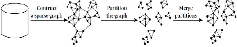
Chameleon [7] is a hierarchical clustering algorithm that uses dynamic modelling to determine the similarity between pairs of clusters In Chameleon, cluster similarity is assessed based on how well-connected objects are within a cluster and on the proximity of clusters. That is, two clusters are merged if their interconnectivity is high and they are close together. Thus, Chameleon does not depend on a static, user-supplied model and can automatically adapt to the internal characteristics of the clusters being merged. The merge process facilitates the discovery of natural and homogeneous clusters and applies to all types of data as long as a similarity function can be specified. The main approach of Chameleon is illustrated in Figure 4.
[image:6.612.330.570.502.550.2]
Fig 4: Hierarchical clustering based on k-nearest neighbours and dynamic modelling
International Journal of Emerging Technology and Advanced Engineering
Website: www.ijetae.com (ISSN 2250-2459, Volume 2, Issue 9, September 2012)509 To determine the pairs of most similar sub-clusters, it takes into account both the interconnectivity as well as the closeness of the clusters. The cluster C is partitioned into sub-clusters Ci and Cj so as to minimize the weight of the edges that would be cut should C be bisected into Ci and Cj. Edge cut is denoted EC (Ci, Cj) and assesses the absolute interconnectivity between clusters Ci and Cj. Chameleon determines the similarity between each pair of clusters Ci and Cj according to their relative interconnectivity, RI (Ci, Cj), and their relative closeness, RC( Ci, Cj): The relative interconnectivity, RI(Ci, Cj), between two clusters, Ci and Cj, is defined as the absolute interconnectivity between Ci and Cj, normalized with respect to the internal interconnectivity of the two clusters, Ci and Cj. That is,
𝑅𝐼 𝐶
𝑖, 𝐶
𝑗=
𝐸𝐶
𝐶𝑖,𝐶𝑗1
2 𝐸𝐶
𝐶𝑖+ 𝐸𝐶
𝐶𝑗where ECCi, Cj is the edge cut, defined as above, for a cluster containing both Ci and Cj. Similarly, ECCi (or ECCj ) is the minimum sum of the cut edges that partition Ci (or Cj) into two roughly equal parts. The relative closeness, RC (Ci, Cj), between a pair of clusters, Ci and Cj, is the absolute closeness between Ci and Cj, normalized with respect to the internal closeness of the two clusters, Ci and Cj. It is defined as
𝐶 𝐶
𝑖, 𝐶
𝑗=
𝑆
𝐸𝐶 𝐶𝑖,𝐶𝑗𝐶
𝑖𝐶
𝑖+ 𝐶
𝑖𝑆
𝐸𝐶𝐶𝑖+
𝐶
𝑗𝐶
𝑖+ 𝐶
𝑖𝑆
𝐸𝐶𝐶𝑗where SECCi; Cj is the average weight of the edges that connect vertices in Ci to vertices in Cj, and SECCi (or SECCj ) is the average weight of the edges that belong to the mincut bisector of cluster Ci (or Cj). Chameleon has been shown to have greater power at discovering arbitrarily shaped clusters of high quality than several well-known algorithms such as BIRCH and density based DBSCAN. However, the processing cost for high-dimensional data may require O (n2) time for n objects in the worst case.
E. DBSCAN
DBSCAN (Density-Based Spatial Clustering of Applications with Noise) [8] is a density-based clustering algorithm. The algorithm grows regions with sufficiently high density into clusters and discovers clusters of arbitrary shape in spatial databases with noise. It defines a cluster as a maximal set of density-connected points. The neighbourhood within a radius e of a given object is called the e-neighbourhood of the object. If the e-neighbourhood
of an object contains at least a minimum number, MinPts, of objects, then the object is called a core object.
Example: Density-reachability and density connectivity. Consider Figure 5 for a given ϵ represented by the radius of the circles, and, say, let MinPts = 3. Based on the above definitions: Of the points, p, o, and r are core objects because each is in an ϵ-neighbourhood containing at least three points. q is directly density-reachable from m. m is directly density-reachable from p and vice versa. q is (indirectly) density-reachable from p because q is directly reachable from m and m is directly density-reachable from p. However, p is not density-density-reachable from q because q is not a core object. Similarly, r and s are density-reachable from o, and o is density-reachable from r. o, r, and s are all density-connected. A density-based cluster is a set of density-connected objects that is maximal with respect to density-reachability. Every object not contained in any cluster is considered to be noise.
Fig 5: Density-reachability and density-connectivity in density-based clustering
Algorithm: DBSCAN: a density-based clustering
algorithm.
Input: D: a data set containing n objects, ϵ: the radius parameter, and
Min Pts: the neighborhood density threshold. Output: A set of density-based clusters.
Method:
1. Mark all objects as unvisited; 2. do
3. randomly select an unvisited object p; 4. mark p as visited;
5. if the ϵ-neighborhood of p has at least Minpts objects
6. create a new cluster C, and add p to C;
7. let N be the set of objects in the ϵ-neighborhood of p;
[image:7.612.326.563.347.460.2]International Journal of Emerging Technology and Advanced Engineering
Website: www.ijetae.com (ISSN 2250-2459, Volume 2, Issue 9, September 2012)510 10. mark p’ as visited;
11. if the ϵ-neighborhood of p’ has at least MinPts points, add those points to N;
12. if p’ is not yet a member of any cluster, add p’ to C; 13. end for
14. output C;
15. else mark p as noise; 16. until no object is unvisited;
DBSCAN searches for clusters by checking the neighbourhood of each point in the database. If the e-neighbourhood of a point p contains more than MinPts, a new cluster with p as a core object is created. DBSCAN then iteratively collects directly density-reachable objects from these core objects, which may involve the merge of a few density-reachable clusters. The process terminates when no new point can be added to any cluster.
If a spatial index is used, the computational complexity of DBSCAN is O(nlogn), where n is the number of database objects. Otherwise, it is O(n2).With appropriate settings of the user-defined parameters e and MinPts, the algorithm is effective at finding arbitrary-shaped clusters.
F. OPTICS: Ordering Points To Identify the Clustering
Structure
Although DBSCAN [10] can cluster objects given input parameters such as e and MinPts, it still leaves the user with the responsibility of selecting parameter values that will lead to the discovery of acceptable clusters. Actually, this is a problem associated with many other clustering algorithms. Such parameter settings are usually empirically set and difficult to determine, especially for real-world, high-dimensional data sets. Most algorithms are very sensitive to such parameter values: slightly different settings may lead to very different clustering of the data. Moreover, high-dimensional real data sets often have very Skewed distributions, such that their intrinsic clustering structure may not be characterized by global density parameters. To help overcome this difficulty, a cluster analysis method called OPTICS was proposed. Rather than produce a data set clustering explicitly, OPTICS computes an augmented cluster ordering for automatic and interactive cluster analysis. This ordering represents the density-based clustering structure of the data. It contains information that is equivalent to density-based clustering obtained from a wide range of parameter settings. The cluster ordering can be used to extract basic clustering information (such as cluster centres or arbitrary-shaped clusters) as well as provide the intrinsic clustering structure.
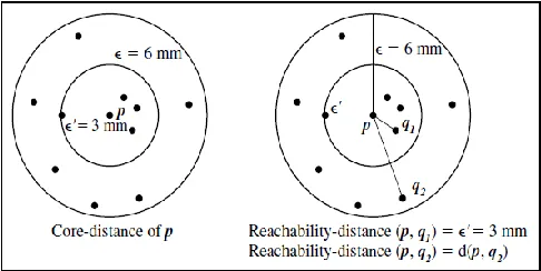
Example: Core-distance and reachability-distance. Figure 6 illustrates the concepts of coredistance and reachability-distance. Suppose that e=6 mm and MinPts=5.
[image:8.612.327.570.218.340.2]The coredistance of p is the distance, e0, between p and the fourth closest data object. The reachability-distance of q1 with respect to p is the core-distance of p (i.e., e0 =3 mm) because this is greater than the Euclidean distance from p to q1. The reachability distance of q2 with respect to p is the Euclidean distance from p to q2 because this is greater than the core-distance of p.
Fig 6: OPTICS terminology
The OPTICS algorithm creates an ordering of the objects in a database, additionally storing the core-distance and a suitable reachability-distance for each object. An algorithm was proposed to extract clusters based on the ordering information produced by OPTICS. Such information is sufficient for the extraction of all density-based clustering with respect to any distance e0 that is smaller than the distance ϵ used in generating the order.
The cluster ordering of a data set can be represented graphically, which helps in its understanding. Methods have also been developed for viewing clustering structures of high-dimensional data at various levels of detail. Because of the structural equivalence of the OPTICS algorithm to DBSCAN, the OPTICS algorithm has the same runtime complexity as that of DBSCAN, that is, O (nlogn) if a spatial index is used, where n is the number of objects.
G. STING: Statistical Information Grid
International Journal of Emerging Technology and Advanced Engineering
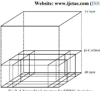
Website: www.ijetae.com (ISSN 2250-2459, Volume 2, Issue 9, September 2012) [image:9.612.68.267.118.299.2]511 Fig 7: A hierarchical structure for STING clustering
Statistical parameters of higher-level cells can easily be computed from the parameters of the lower-level cells. These parameters include the following: the attribute-independent parameter, count; the attribute-dependent parameters, mean, stdev (standard deviation), min (minimum), max (maximum); and the type of distribution that the attribute value in the cell follows, such as normal, uniform, exponential, or none (if the distribution is unknown).When the data are loaded into the database, the parameters count, mean, stdev, min, and max of the bottom-level cells are calculated directly from the data. The value of distribution may either be assigned by the user if the distribution type is known beforehand or obtained by hypothesis tests such as the c2 test. The type of distribution of a higher-level cell can be computed based on the majority of distribution types of its corresponding lower-level cells in conjunction with a threshold filtering process. If the distributions of the lower level cells disagree with each other and fail the threshold test, the distribution type of the high-level cell is set to none. STING offers several advantages: (1) the grid-based computation is query-independent, because the statistical information stored in each cell represents the summary information of the data in the grid cell, independent of the query; (2) the grid structure facilitates parallel processing and incremental updating; and (3) the method’s efficiency is a major advantage: STING goes through the database once to compute the statistical parameters of the cells, and hence the time complexity of generating clusters is O(n), where n is the total number of objects. After generating the hierarchical structure, the query processing time is O(g), where g is the total number of grid cells at the lowest level, which is usually much smaller than n. Because STING uses a multi-resolution approach to cluster analysis, the quality of STING clustering depends on the granularity of the
lowest level of the grid structure. If the granularity is very fine, the cost of processing will increase substantially; however, if the bottom level of the grid structure is too coarse, it may reduce the quality of cluster analysis. As a result, the shapes of the resulting clusters are isothetic; that is, all of the cluster boundaries are either horizontal or vertical, and no diagonal boundary is detected. This may lower the quality and accuracy of the clusters despite the fast processing time of the technique.
H. CLIQUE:CLustering InQUEst
CLIQUE [10] was the first algorithm proposed for dimension-growth subspace clustering in high-dimensional space. In dimension-growth subspace clustering, the clustering process starts at single-dimensional subspaces and grows upward to higher-dimensional ones. Because CLIQUE partitions each dimension like a grid structure and determines whether a cell is dense based on the number of points it contains, it can also be viewed as an integration of density-based and grid-based clustering methods. However, its overall approach is typical of subspace clustering for high-dimensional space, and so it is introduced in this section.
The ideas of the CLIQUE clustering algorithm are outlined as follows.
1. Given a large set of multidimensional data points, the data space is usually not uniformly occupied by the data points. CLIQUE’s clustering identifies the sparse and the ―crowded‖ areas in space (or units), thereby discovering the overall distribution patterns of the data set.
2. A unit is dense if the fraction of total data points contained in it exceeds an input model parameter. In CLIQUE, a cluster is defined as a maximal set of connected dense units.
International Journal of Emerging Technology and Advanced Engineering
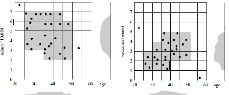
Website: www.ijetae.com (ISSN 2250-2459, Volume 2, Issue 9, September 2012) [image:10.612.52.286.140.238.2]512 Fig 8: Dense units found with respect to age for the dimensions salary and vacation are intersected to provide a candidate search space for the dense units of higher dimensionality
The subspaces representing these dense units are to form a candidate search space in which dense units of higher dimensionality may exist. In the second step, CLIQUE generates a minimal description for each cluster as follows. For each cluster, it determines the maximal region that covers the cluster of connected dense units. It then determines a minimal cover (logic description) for each cluster. CLIQUE automatically finds subspaces of the highest dimensionality such that high-density clusters exist in those subspaces. It scales linearly with the size of input and has good scalability as the number of dimensions in the data is increased. However, obtaining meaningful clustering results is dependent on proper tuning of the grid size and the density threshold.
This is particularly difficult because the grid size and density threshold are used across all combinations of dimensions in the data set. Thus, the accuracy of the clustering results may be degraded at the expense of the simplicity of the method. Moreover, for a given dense region, all projections of the region onto lower dimensionality subspaces will also be dense. This can result in a large overlap among the reported dense regions. Furthermore, it is difficult to find clusters of rather different density within different dimensional subspaces.
V. CONCLUSION
In this paper we have studied a significant functionality of data mining that is, clustering analysis. As mentioned earlier clustering analysis is to find the intrinsic structures in data, and organize them into small subgroups, clusters for further analysis. Clustering is done on the basis of similarity and dissimilarity measures using different notations like distance measures, density measures. In this paper four clustering methods are discussed, partitioning method which uses distance measure to find mutually exclusive cluster of spherical shaped on small-to-medium data sets.
In hierarchical method clustering is done on hierarchical decomposition of data. Major drawback of this method once a step is done it can never be undone. To overcome this multiphase clustering is used by BIRCH or chameleon.
Density-based clustering method can find arbitrary shaped cluster by using density as a notation. This method may filter out outliers. It grows cluster according to density of neighbourhood objects like in DBSCAN. Optics creates an augmented ordering of data’s clustering structures. Grid based methods used multiresolution grid data structure. It provides fast processing time. STING is a typical example of a grid based method on statistical information stored in grid cells. CLIQUE is a grid based and subspace clustering algorithm.
All clustering algorithm are generates cluster, but just vary from each other due to similarity measure, size of data set, static or dynamic data set, and most important shape of clusters. Many extensions of these algorithms are available in literature to enhance clustering analysis for further studies of data mining.
REFRENCES
[1] X. Wu, V. Kumar, J.R. Quinlan, J. Ghosh, Q. Yang, H. Motoda, G.J. McLachlan, A. Ng, B. Liu, P.S. Yu, Z.-H. Zhou, M. Steinbach, D.J.Hand, and D. Steinberg, ―Top 10 Algorithms in Data Mining, ―Knowledge Information Systems, vol. 14, no. 1, pp. 1-37, 2007 [2] I. Guyon, U.V. Luxburg, and R.C. Williamson, ―Clustering: Science
or Art?,‖ Proc. NIPS Workshop Clustering Theory, 2009.
[3] Berkhin, P.,‖ Survey of clustering data mining techniques.‖, technical-report,2002
www.ee.ucr.edu/~barth/EE242/clustering_survey.pdf
[4] Tapas Kanungo, , David M. Mount, Nathan S. Netanyahu, Christine D. Piatko, Ruth Silverman, and Angela Y. Wu,‖ An Efficient k-Means Clustering Algorithm:Analysis and Implementation.‖, IEEE TRANSACTIONS ON PATTERN ANALYSIS AND MACHINE INTELLIGENCE, VOL. 24, NO. 7, JULY 2002
[5] Umadevi Chezhian, Thanappan Subhash. M. Raghvan, ―Hierarchical Sequence Clustering Algorithm for Data Mining‖, Proceedings of the World Congress on Engineering 2011 Vol III WCE 2011, July 6 - 8, 2011, London, U.K
[6] T. Zhang, R. Ramakrishnan, and M. Livny. BIRCH: an efficient data clustering method for very large databases. Proc. 1996 ACM-SIGMOD Int. Conf. Management of Data, pp. 103-114, Montreal, Canada, June 1996
International Journal of Emerging Technology and Advanced Engineering
Website: www.ijetae.com (ISSN 2250-2459, Volume 2, Issue 9, September 2012)513 [8] Ester M., Kriegel H.-P., Sander J. and Xu X, ―A Density-Based
Algorithm for Discovering Clusters in Large Spatial Databases with Noise‖, Proc. 2nd Int. Conf. on Knowledge Discovery and Data Mining, 1996.
[9] Wei Wang, Jiong Yang, and Richard Muntz : STING : A Statistical Grid Appraoch to Spatial Data Mining : Department of Computer Science, University of California, Los Angels