Free Vibration Analysis of a Rotating Non-Uniform Blade
with Multiple Open Cracks Using DQEM
K. Torabi
1, H. Afshari
1, M. Heidari-Rarani
2,*1Faculty of Mechanical Engineering, University of Kashan, Kashan, 87317-51167, Iran
2Department of Mechanical Engineering, Faculty of Engineering, University of Isfahan, 81746-73441, Isfahan, Iran *Corresponding Author: [email protected]
Copyright © 2014 Horizon Research Publishing All rights reserved.
Abstract
In this paper, differential quadrature element method (DQEM) is used to analyze the free transverse vibration of a multiple cracked non-uniform Timoshenko blade rotating with a constant angular velocity. The blade’s deflection is assumed to be small so that the nonlinear terms can be neglected. Governing equations, compatibility conditions at the damaged cross-sections and boundary conditions are derived and formulated by the differential quadrature rules. First, the precision of the proposed method is confirmed by the exact solutions available in the literature. Then, the effect of angular velocity value as well as the location, depth and numbers of the cracks are investigated on the natural frequencies of the blade. The advantages of the proposed method are applicable for blades with any arbitrary variable section and less time-consuming for cases with several cracks.Keywords
DQEM, Transverse Vibration, Crack, Rotating Blade1. Introduction
Existence of cracks causes to abrupt failure in structures and sometimes is difficult to be detected. Depended on the position and extension of the cracks, eigen parameters of the structure would be affected and it can be used as a non-destructive method to detection of the damages in the structure. Using vibration based detection methods has been one of the most important challenges confronting active research in the last decade. Several authors have proposed techniques to estimate the effects of damage on the eigen parameters of a structure (usually known as the direct problem), while others have dealt with the problem of detecting, locating and quantifying the extent of damage (well-known as the inverse problem). A few authors have addressed aspects concerning the identification of the cracks, leading to explicit expressions for the solution of the inverse problem [1]. Also, variation of the natural frequencies with the depth and position of a concentrated crack has been
explained in the references such as Morassi [2, 3] and Narkis [4]. During the recent years, more attention has been dedicated to the solution of the direct analysis problem of vibrating beams in the presence of multiple cracks. Some research works have introduced the concentrated cracks on the beams by considering a local reduction of the flexural stiffness. According to this model, a crack can be represented as an elastic link connecting the two adjacent beam segments. In other words, it is modeled as a mass-less rotational spring whose stiffness is dependent on the extent of the damage. The first studies were based on the division of the beam into sub-beams between two consequent cracks [5, 6].
In most of the studies, the beam is considered as a slender one which can be analyzed by Euler-Bernoulli beam theory. Thus, shear deformation and rotary inertia of the beam are neglected. Recently, some authors have focused on vibration analysis of the cracked short beams which are modeled by Timoshenko beam theory. Zheng and Fan [7] used modified Fourier series to investigate vibration of the cracked Timoshenko beams with different boundary conditions. Lele and Maiti [8] proposed a new method based on the Timoshenko beam theory considering shear effects. In this method, the characteristic equation to obtain the natural frequencies for the cantilever cracked beam is expressed as an eighth-order determinant equated to zero. Lin [9] presented a closed-form solution for prediction of natural frequencies of a cracked simply supported Timoshenko beam. Using transfer matrix technique, Khaji et al. [10] introduced a closed-form solution for crack detection problem of Timoshenko beams for the various boundary conditions.
on modal and elastic wave propagation analysis of a cracked Timoshenko beam. Loya et al. [12] obtained natural frequencies for bending vibrations of a simply supported cracked Timoshenko beam with simple expressions for the natural frequencies.
The DQM is a numerical approach for solving the differential equations which was initially introduced by Bellman et al. [13], and further was developed by Bellman and Roth [14]. Bert and his co-workers [15-20], contributed to the development of the method and used the DQM for the analysis of the structural problems. This method can be applied only for continuous problems. Hence, DQM was promoted to use for problems with local discontinuities. Recently, differential quadrature element method (DQEM) has appeared as a numerical technique for analyzing the structures with some local discontinuities in loading, material properties and geometry. Thus, this method is applied to solve many problems especially in the vibration analysis. Chen [21-24] solved different vibration problems using DQEM. E.g., he studied about the vibration of non-uniform shear deformable axisymmetric orthotropic circular plates [21], vibration analysis of non-prismatic shear deformable beams resting on elastic foundations [22], in-plane vibration of curved beam structures [23], and out-of-plane vibration of non-prismatic curved beam structures regarding the effect of shear deformation [24]. Malekzadeh et al. [25] presented a semi-analytical solution for the free vibration analysis of thick plates with the two opposite edges simply supported using DQEM. DQEM was hired by Torabi et al. [26] for free vibration analysis of a non-uniform cantilever Timoshenko beam with multiple concentrated masses. Torabi et al. [27] employed DQEM to analyze the free transverse vibration of multiple cracked non-uniform Timoshenko beams with general boundary conditions.
In this paper, DQEM is used to analyze free transverse vibration of a damaged non-uniform Timoshenko blade. Therefore, the accuracy of the proposed DQEM is first confirmed by the exact solutions available in the literature for the uniform Timoshenko beam. Then, the effect of location, depth and numbers of the cracks as well as the angular velocity of blade are investigated on the natural frequencies.
2. Differential Quadrature Method
In the differential quadrature method (DQM), all derivatives of a function are approximated by means of the weighted linear sum of the functions values at a pre-selected grid of discrete points as
( )
1
,
i
r N
r ij j r
j x x
d f
A f
dx
= ==
∑
(1)where N is the number of grid points in the x-direction. In Eq. (1), A(r) is the weighting coefficient associated with the rth
order derivative. This matrix is given for the first-order derivative as [18]
(1) 1
,
1
1
( )
, ( , 1,2,3,..., ; )
( ) ;
1 , ( 1,2,3,..., )
( )
N
i m m
m i j N
j m ij m
m j N
m i m
m i
x x
i j N i j
x x
A
i j N
x x
= ≠ = ≠ = ≠
−
= ≠
−
=
= =
−
∏
∏
∑
(2)
For higher-order derivatives, this matrix can be obtained from a recursive relation as A(r)=A(1)A(r-1). In addition to
number of grid points, distribution of them is an important factor in convergence of solution. A well-accepted set of the grid points is the Gauss–Lobatto–Chebyshev points given for interval [0,1] by
1 1 cos[( 1) ] , ( 1,2,3,..., ).
2 ( 1)
i i
x i N
N
π
−
= − − =
(3)
3. Vibration Analysis of a Damaged
Non-Uniform Timoshenko Blade
3.1. Governing Equations
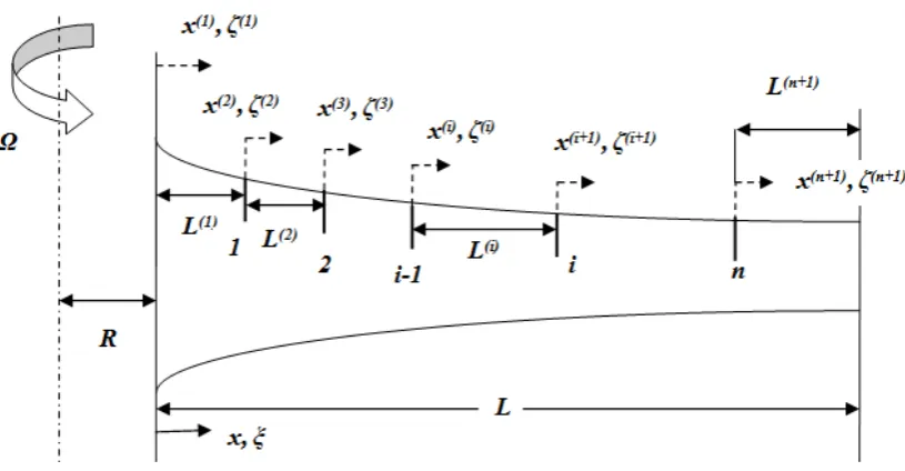
As depicted in Fig. 1, a rotating non-uniform Timoshenko blade with multiple open cracks is considered. The governing equations for free vibration of an intact beam rotating with constant angular velocity can be written as [28]
2 2
2 2
2
( , )
( ) ( , )
( , ) ( , )
( ) ( ) 0
,
( , ) ( , )
( ) ( ) ( , )
( , )
( ) ( , ) ( ) 0
w x t
kGA x x t
x x
w x t w x t
T x A x
x x t
x t w x t
EI x kGA x x t
x x x
x t
I x x t I x
t
ψ
ρ
ψ ψ
ψ
ρ ψ ρ
∂ ∂ − +
∂ ∂
∂ ∂ − ∂ =
∂ ∂ ∂
∂ ∂ + ∂ −
∂ ∂ ∂
∂
+ Ω − =
∂
(4)
Figure 1. Non-uniform Timoshenko blade with multiple open cracks.
( ) (
2)
( ) xL ,
T x =
∫
ρA x Ω R x dx+ (5) Applying separation of variables method, the displacement w(x,t) and rotation due to bending ψ(x,t) can be assumed as( , )
( )
i t,
( , )
( )
i tw x t
=
W x e
ωψ
x t
= Ψ
x e
ω (6)where ω is angular natural frequency of vibration. In order to obtain the dimensionless form of cross-sectional area and the second moment of inertia, these values are divided into the cross-sectional area and second moment of inertia of the beam at the clamped edge.
( )
( )
( )
( )
* *
0 0
, .
A x I x
A x I x
A I
= = (7)
Substituting Eqs. (5)-(7) into the Eq. (4), the following set of differential equations obtain:
(
) ( )
(
)
2 *
2 *
*
2 2
* 2
2 2
( ) ( ) 1 ( ) ( ) ( )
( )
( ) ( )
( ) ( ) 0
L x
d W x d x dA x dW x x
dx dx dx
dx A x
R x A x dx d W x
kG A x dx
R x dW x W x
kG dx kG
ρ
ρ ρω
Ψ
− + − Ψ
+ Ω
+
Ω +
− + =
∫
2 *
0
2 *
0 * *
2 2
0 0
0 0
( ) 1 ( ) ( )
( )
( ) ( ) ( )
( )
( ) ( ) 0,
EI d x dI x d x
kA G dx I x dx dx
A x dW x x
dx I x
I I
x x
kA G kA G
ρ ρ ω
Ψ + Ψ
+ − Ψ
Ω
+ Ψ + Ψ =
(8)
For the ith sub-beam, Eq. (8) can be written as
( )
( )
( )
( )
( )
(
) ( )
( )
( )
(
)
( )
( )
( )
( )
2 ( ) ( ) ( ) ( )
2 ( )
( )
( ) ( ) *
( ) ( )
* ( )
* 2 ( ) ( )
2
* ( ) 2
( ) ( )
2 2
( ) ( ) ( )
2 ( ) ( ) * ( ) (
0
2 *
( ) 0
1 ( )
( )
( )
0
1 ( )
( )
i i i i
i i
i i
i i i
L i i
x
i i i
i i i
i i i i
i
d W x d x
dx d x
dW x
dA x x
dx
A x dx
R x A x dx d W x
kG A x d x
dW x
R x
W x
kG dx kG
d x d x
EI dI x
kA G d x I x dx
ρ
ρ ρω
Ψ −
+ − Ψ
+ Ω
+
Ω +
− + =
Ψ Ψ
+
∫
( )
( )
( )
( )
( )
) ( )
( ) ( ) *
( ) ( )
* ( )
2 2
( ) ( ) ( ) ( )
0 0
0 0
.
( ) ( )
0
i i i
i i i
i i i i
dx
dW x
A x x
I x dx
I x I x
kA G kA G
ρ ρ ω
+ − Ψ
Ω
+ Ψ + Ψ =
(9)
By introducing the following dimensionless parameters:
( ) ( )
( ) ( ) ( )
( ) ( )
2 0 2 0
2 2
0 0
4 2 4 2
4 0 4 0
0 0
,
i i i
i i i
i
x
v
W
l
L
L
L
L
I
EI
x
r
s
L
A L
kGA L
A L
A L
R
L
EI
EI
ζ
ξ
ρ
ρ
ω
δ
γ
λ
=
=
=
=
=
=
Ω
=
=
=
(10)
( )
( )
( )
( )
( )
( )( )
( )
( )
( )
2 ( ) ( ) ( ) ( )
2
( ) ( ) 2 ( ) ( )
( ) ( ) *
( ) ( )
* ( ) ( )
1 *
2 ( ) ( ) ( ) ( )
2 4 2
* ( ) ( ) 2 ( ) ( )
4 2 ( ) ( )
2
1 1
1 ( ) 1
( )
( ) 1
( )
0
1
i i i i
i i i i
i i
i i i i
i i i i
i i i i
i i
d v d
l d l d
dv dA
d
A l d
A d d v dv
s
A l d l d
s v s ξ ζ ζ ζ ζ ζ ξ ζ ξ ξ ζ
ξ δ ξ ξ ζ δ ξ ζ
γ
ξ ζ ζ
λ ζ Ψ −
+ − Ψ
+ + + − + =
∫
( )
( )
( )
( )
( )
( )
( )
2 ( ) ( ) ( ) ( )
2 *
( ) ( ) 2 * ( ) ( )
( ) ( ) *
( ) ( )
* ( ) ( )
4 2 2 ( ) ( ) 4 2 2 ( ) ( )
.
1 ( ) 1 ( )
( ) 1 ( )
0
i i i i
i i i i
i i
i i i i
i i i i
d dI d
d
l d I l d
dv A
I l d
s r s r
ζ ξ ζ
ξ ξ ζ ζ ζ ξ ζ ξ ζ
γ ζ λ ζ
Ψ Ψ
+
+ − Ψ
+ Ψ + Ψ =
(11) By considering the equal number of grid points for all sub-beams, it can be clearly expressed that
( )1 ( )2 ( )3
...
( )i...
(n 1),
ζ
=
ζ
=
ζ
= =
ζ
= =
ζ
+=
ζ
(12)hence, Eqs. (11) can be simplified as
( )
( )
( )
( )
(
)
( )
( )
( )
( )
2 2 ( ) ( )
( ) 2 ( )
( ) *
( )
* ( )
1 *
2 2 ( ) ( )
4 2
* ( ) 2 ( )
4 2 ( )
2 2 ( ) *
2
( ) 2 *
1 1
1 ( ) 1
( )
( ) 1
( )
0
1 1 ( )
( ) i i i i i i i i i i i i i i
d v d
d
l d l
dv dA
d d
A l
A d d v dv
s
d
A l d l
s v
d dI
s d
l d I
ξ ζ ζ ζ ζ ζ ξ ζ ξ ζ ξ
ξ δ ξ ξ ζ δ ξ ζ
γ ζ ξ ζ λ ζ ζ ξ ξ ζ ξ Ψ −
+ − Ψ
+ + + − + = Ψ +
∫
( )
( )
( )
( )
( )
( ) ( ) ( ) * ( ) * ( )4 2 2 ( ) 4 2 2 ( )
.
1
( ) 1 ( ) 0 i i i i i i i d d l dv A d I l
s r s r
ζ ζ ζ ξ ζ ζ ξ
γ ζ λ ζ
Ψ
+ − Ψ
+ Ψ + Ψ =
(13) It should be stated that in this paper, in order to simplify the DQ analogue, a modified form of the weighting coefficients of ith sub-beam are defined as
( ) ( )
( )
1 2
( ) ( )
( ) ( ) 2
[ ] [ ]
[ ]i , [ ]i ,
i i
A A
A B
l l
= = (14)
Hence, the DQ analogue of the governing set of equations of element “i” becomes
[ ]
{ }
[ ]
{ }
{ }
[ ]
{ }
[ ]
{ }
{ }
( ) ( ) ( ) ( ) 4 2 ( )
( ) ( ) ( ) ( ) 4 2 2 ( )
0 , 0
i i i i i
ve se
i i i i i
se ve
B v A s v
B A v s r
λ λ
+ Ψ + =
Ψ + + Ψ =
(15) where
[ ]
[ ]
[ ] [ ]
(
[ ] [ ]
[ ] [ ]
)
[ ]
[ ] [ ]
[ ]
(
[ ]
[ ] [ ]
)
[ ]
[ ]
[ ] [ ]
( ) ( ) ( ) ( ) 4 2 ( ) ( ) ( ) ( )
( ) ( ) ( )
( ) 2 ( ) ( ) ( ) 4 2 ( )
( ) ( ) ( )
.
i i i i i i i i
ve
i i i
se
i i i i i
se
i i i ve
B B a A s b B c A
A A a
B s B d A r I e
A e A
γ γ = + + + = − − = + + − = (16) In the last equation, [a](i), [b](i),...,[e](i) are diagonal
geometry-dependent matrices defined as
( ) ( ) ( ) ( ) ( ) ( ) ( ) ( ) ( ) 1 * * * * * * * * ( )
1 ( )
( ) ( )
1 ( ) .
( ) 1,2,..., 1
( ) 1,2,..., N
( )
1 1,2,..., 1
m m m i i jj jj m i i
jj m jj
i m jj m A d dA a b d A A dI c d d I i n A e j
I m i N j n N
ξ ξ ξ
ξ ξ
ξ δ ξ ξ ξ ξ ξ ξ ξ δ ξ ξ ξ ξ ξ = = + = = = − + = = + = = = − + = +
∫
(17)As mentioned in Refs. [29-31], in order to eliminate the redundant equations, the equations of motion should be written just for the domain points. Therefore, Eq. (15) should be represented as
{ }
{ }
{ }
{ }
{ }
{ }
( ) ( ) ( ) ( ) ( ) 4 2
( ) ( ) ( ) ( ) ( ) 4 2 2
0 . 0 i
i i i i
ve se
i
i i i i
se ve
B v A s v
B A v s r
λ
λ
+ Ψ + =
Ψ + + Ψ =
(18)
In Eq. (18), bar signs show the corresponded truncated non-square matrices. By combination of element equations, the following relations yield
[ ]
{ }
[ ]
{ }
{ }
[ ]
{ }
[ ]
{ }
{ }
4 2
4 2 2
0 , 0
v s d
s v d
B v A s v
B A v s r
λ
λ
+ Ψ + =
Ψ + + Ψ = (19)
where
{ }
{ }
(1) (2) ( 1)
1 1 1
(1) (2) ( 1)
2 2 2
(1) (2) ( 1)
1 1 1
(1) (2) ( 1)
1
. . .
. . . .
. . .
T
T T n T
n
n
N N N
n
N N N
v v v
v v v
v
v v v
v v v
+ + + − − − + = Ψ Ψ =
(1) (2) ( 1)
1 1
(1) (2) ( 1)
2 2 2
(1) (2) ( 1)
1 1 1
(1) (2) ( 1)
. . .
. . . .
. . .
T
T T n T
n
n
N N N
n
N N N
+ +
+
− − −
+
Ψ Ψ
Ψ Ψ Ψ
Ψ Ψ Ψ
Ψ Ψ Ψ
(1) (2) ( ) ( 1) (1) (2) ( ) ( 1)
0 . . 0 0
0 . . 0 0
. . . .
[ ]
. . . .
0 0 . . 0
0 0 . . 0
0 . . 0 0
0 . . 0 0
. . . .
[ ]
. . . .
0 0 . . 0
0 0 . . 0
se se s n se n se ve ve v n ve n ve B B B B B A A A A A + + = = As mentioned in Ref. [32], Eq. (19) may be rearranged in order to separate the boundary, domain, and adjacent displacement and rotation components as
[ ] { } [ ] { } [ ] { } [ ] { }
[ ] { } [ ] { }
{ }
[ ] { } [ ] { } [ ] { } [ ] { }
[ ] { } [ ] { }
{ }
4 2
4 2 2
0
,
0
v b b v d d v c c s b b
s d d s c c d
v b b v d d v c c s b b
s d d s c c d
B
v
B
v
B
v
A
A
A
s v
A
v
A
v
A
v
B
B
B
s r
λ
λ
+
+
+
Ψ
+
Ψ +
Ψ +
=
+
+
+
Ψ
+
Ψ +
Ψ +
Ψ =
(21) where
{ }
{ }
{
}
{ }
{ }
{
}
(1) (1) 1 1( 1) ( 1)
b n b n
N N
v
v
v
+ +
Ψ
=
Ψ =
Ψ
(22){ }
{ }
{
}
{ }
{
}
{
}
(1) (1) (2) (2) 1 1 (2) (2) (3) (3) 1 1 (3) (3) ( ) ( ) 1 1 ( ) ( )( 1) ( 1)
1 1 . . . . . . N N N N N N c c n n n n N N n n v v v v v v v v
v + +
Ψ
Ψ
Ψ
Ψ
Ψ
= Ψ =
Ψ
Ψ
Ψ
.
{ }
{ }
(1) (1) 2 2 (1) (1) 1 1 (2) 2 (2) 1 ( 1) 2 ( 1) 1 . . . . . . . . . . . . . . . N N d d N n n N v v v v v v v − − − + + − Ψ
Ψ
= Ψ =
(2) 2 (2) 1 ( 1) 2 ( 1) 1 . . . . . . . . . N n n N − + + −
Ψ Ψ
Ψ
Ψ
3.2. Compatibility Conditions
Compatibility conditions at common nodes of two adjacent sub-beam in the vicinity of each crack (x=xc), are
continuity in natural parameters and discontinuity in the geometrical parameters as
( ) ( )
( )
( )
( )
( )
( )
( ) ( )
( )
,( ) ( )
c c c c
c c q c
c c m c
q m
V x V x M x M x
W x W x C V x
x h h C x C q C EA EI M x α α + + − − − + − + + + = = − = Ψ
= = Θ
− Ψ = (23)
where h is height of the beam, Ɵ(α) and q(α) are functions of the ratio of the crack depth to the beam height (α) and depend on the beam cross-section geometry. Also, M and V are bending moment and shear force, respectively and are
(1) (2) ( ) ( 1) (1) (2) ( ) ( 1)
0 . . 0 0
0 . . 0 0
. . . .
[ ]
. . . .
0 0 . . 0
0 0 . . 0
0 . . 0 0
0 . . 0 0
. . . .
[ ]
. . . .
0 0 . . 0
0 0 . . 0
presented for ith sub-beam as [28]
( )
( ) ( ) ( ) ( ) ( ) ( ) ( ) ( ) ( ) , i i i i i i i i i d M EI dx dW dWV kAG T x
dx dx
Ψ =
= Ψ − −
(24)
Which can be rewritten using Eqs. (5) and (10) as
( )( ) ( ) ( ) ( ) ( ) ( ) ( ) ( * 4 ) * ) 2 ( . 1 1 1 i i i i i i L i EI d M
L l d
dv V kAG A d d s l A ξ ξ ζ δ ξ ξ ξ ζ γ + Ψ =
= Ψ − +
∫
(25)For a rectangular cross-section, the value of θ(α) and q(α) have been presented respectively, by Tada et al. [34] and Valiente et al. [35] as
2 2
3 4
2 2
3 4
5.93 19.69 37.14 ( ) 2
1 35.84 13.12
; 0.22 3.82 1.54 ( )
1 14.64 9.60
q
α α
α α
α α α
α α
α α
α α α
− +
Θ = − − +
− + + = − − + (26) Using Eqs. (17), (25) and (26), Eq. (23) can be rewritten in the DQ form as
{ }
{ }
{ }
{ }
{ }
{ }
( ) ( 1) ( ) ( ) ( 1 ( ) ( ) ( ) ) ) ( 1 0 [ ] , [ ] [ ] 0 0 0 i i i i i iv i s i i
v p q v q + + +
Ψ
= Ψ
Ψ
+ = Ψ (27) where ( ) ( ) ( ) ( ) ( ) ( ) ( ) ( ) ( ) ( ) ( ) ( ) ( ) ( ) ( ) ( ) 1 1 1 2 4 1 2 4 1 1 1 11 1,1
1, 1 2
2,1
2, 1 2
1,1
1, 1 2
[ ] 2, 2 2 1 , 1 1 1 i Nk i k i jk i NN i i v N i i m Nk Nk
k N i Nk i k N i i
q Nk Nk jk
k N
j k N
j N k N
p
j k N
j N k N
j k N
j N k N
q
j k N
j A
A A
s b A
s b A k N A N χ δ δ γ γ χ δ δ + − − + − + − = ≤ ≤ = + ≤ ≤ = = ≤ ≤ = + ≤ ≤ − − + − = ≤ ≤ = + ≤ ≤ = = ≤ ≤ − + − + ≤ ≤ + = + − ( ) ( ) . 1, 1, 1 [ ] 2 1 , 1 0 i s i q jk
j k N
j k N
q
j k N
else χ = = = = + = − = = − (28)
where dimensionless parameters in Eq. (28) are defined as:
( )
( )
( )( )
(
)
( ) ( )
( ) ( ).
2 1
i i i i i i
m q
h h k q
L L
ξ ξ
χ α χ α
υ
= Θ =
+ (29)
Composing Eqs. (27) for all sub-beams yields
{ } { }
{ }
{ } { }
[ ]P Ψ = 0 [Qv]v +[ ]Qs Ψ = 0 , (30) where [ ] [ ] [ ] [ ] [ ] [ ] [ ] [ ] [ ] [ ] [ ] (1) (2) ( ) ( 1) (1) (2) ( ) ( 1) (1) (2)
0 . . 0 0
0 . . 0 0
. . . .
[ ] . . . . . .
0 0 . . 0
0 0 . . 0
0 . . 0 0
0 . . 0 0
. . . .
[ ] . . . . . .
0 0 . . 0
0 0 . . 0
0 . . 0 0
0 . . 0 0
. . . .
[ ] . . . . . .
0 0 . .
n n v v v n v n v s s s s P P P P P q q Q q q q q Q q + + = = = [ ] ( ) ( 1) . 0
0 0 . . 0
n n s q + (31)
Similar to the procedure done for Eqs. (19) and (21), Eq. (30) can be partitioned as
{ }
{ }
{ } { }
{ }
{ }
{ }
{ }
{ }
{ } { }
[ ] [ ] [ ] 0
[ ] [ ] [ ] .
[ ] [ ] [ ] 0
b d
b b d c
c
b d
d c
v b v d v c
s b s d s c c
P P P
Q Q Q
Q
v v
Q Q
v
+ +
Ψ + Ψ + Ψ
+ Ψ + Ψ + Ψ =
=
(32)
From Eq. (28) and (31), it is obvious that [Qs]b=[0] and [Qs]d=[0]. Hence, Eq. (33) leads to
{ }
{ }
{ }
{ }
[ ]
vb{ }
[ ]
[ ]{ }
[ ]
[ ]{ }
[ ]
{ }
,b d
c b d
vd sb sd
c b d b d
v R v R v R
J J
R
=
Ψ = Ψ + Ψ
+ + Ψ + Ψ (33)
in which
[ ]
[ ]
[ ]
[ ] [ ]
[ ]
1 1 1 1 1 1 [ ] [ ] [ ] [ ] [ ] [ ] [ ] [ ] [ ] [ ] . [ ] [ ] [ ] [ ]b c b d c d
v c v b v c
vb v d
v c s c b v c s c
sb d
vd sd
J P P J P P
Q Q Q Q
Q
R R
R Q J R Q Q J
− − − − − − = − = − = − = − = − = − (34)
Substituting Eq. (33) into Eq. (21), next set of equations can be extracted as
{ }
{ }
{ }
{ }
{ }
{ }
{ }
{ }
{ }
{ }
4 2
4 2 2
[ ] [ ] [ ]
[ ] 0
,
[ ] [ ] [ ]
[ ] 0
v b b v d d s b b
s d d d
s b b s d d v b b
v d d d
G v G v G
G s v
E E E v
E v s r
λ
λ
+ + Ψ
+ Ψ + =
Ψ + Ψ +
+ + Ψ =
(35) where
[ ]
[ ]
[ ]
[ ]
[ ]
[ ]
[ ]
[ ]
[ ]
[ ]
[ ]
[ ]
[ ] [ ] [ ] [ ] [ ] [ ] [ ] [ ] [ ] [ ] [ ] [ ] [ ] [ ] . [ ] [ ] [ ] [ ] [ ] [ ] [ ] [ ] [ ] [ ] [ ] [ ] [ ] [ ]v b v b v c
v d v d v c
s b v c s b s c b
s d v c s d s c d
s b s b s c b v c
s d s d s c d v
vb
c
v b v b v
vd sb sd sb sd vb c
v d v d v c vd
G B B
G B B
G B A
R R R R R A J
G B A
R R
A J
E B B J A
E B B J A
E A A
E A A R
= + = + = + = + = + + = + + = + = + +
3.3. Boundary Conditions
Since a rotating blade acts as a cantilever beam, boundary conditions can be defined as
( ) ( )
( ) ( ) ( )
( ) ( )
( )
( ) ( )
1 1
1 1 1 1
1 1
0 0
1 1
0 0
.
0 0
n n n n
x x
n n
x L x L
W
M V
ψ
+ + + +
= =
+ +
= =
= =
= = (37)
Eq. (37) can be rewritten using Eq. (25) as ( )
( )
( ) ( )
1 1
1 1
0 0
(n 1) (n 1)
(n 1) ( )
1
( )
1
0 0
.
0 0
1 1
x x
i i
d dv
d d
l l
v
ζ ζ
ζ ζ
= =
=
+ +
= +
Ψ − Ψ
=
= Ψ =
= (38)
DQ form of Eq. (38) can be indicated as
[ ]
m
{ }
Ψ =
0
,
[ ]
m
{ }
v
+
[ ]
z
{ } { }
Ψ =
0
,
(39) where( )
( )
(
)
(
)
(
)
1
1 1
2, 1 1
0
1 2, 1
. 0
1,2 1 1
jk
jk n N k nN
j k
m j nN k n N
else
j k n N
z
else
j k n N
A +
−
= =
= = + ≤ ≤ +
− = = +
=
= ≤ ≤ +
(40)
Again, Eq. (39) may be partitioned as
{ }
{ }
{ } { }
{ }
{ }
{ }
{ }
{ }
{ } { }
[ ]
[ ]
[ ]
0
[ ]
[ ]
[ ]
.
[ ]
[ ]
[ ]
0
b b d d c c
b d c
b
b d c
b d d c c
v
v
m
m
m
v
m
m
m
z
z
z
Ψ +
Ψ +
Ψ
+
+
+
Ψ +
Ψ +
Ψ =
=
(41)
From Eq. (40), it can be found that [z]c=[0] and [z]d=[0];
Therefore, using Eq. (33), Eq. (41) can be written as
{ }
Ψ b =[ ]t{ } { }
Ψ d v b =[ ]hv{ }
v d +[ ]hs{ }
Ψ d, (42) where(
) (
)
(
) (
)
(
)
(
)
[ ]
1
1
1
[ ] [ ] [ ] [ ] [ ] [ ] [ ]
[ ] [ ] [ ] [ ] [ ] [ ] [ ] .
[ ] [ ] [ ] [ ] [ ] [ ]
[ ] [ ] [ ]
b c b d c d
v b c vb d c vd
c sd
s b c vb
b c sb
t m m J m m J
h m m R m m R
m R
h m m R z m R t
− − −
= − + +
= − + +
= − + + +
(43)
Replacing Eq. (42) into the Eq. (35), the following eigenvalue equation obtain:
[ ]{ }
4[ ]{ }
,d d
K u =
λ
M u (44) where{ }
{ }
{ }
[ ]
[ ]
[ ]
[ ]
( )( )[ ]
( )( )[ ]
( )( ) ( )( )1 2 1 2
2
2
1 2
1 2
[ ][ ] [ ] [ ] [ ] [ ][ ]
.
[ ][ ] [ ] [ ] [ ] [ ][ ]
0 0
d d
d
vb v vd sb sd vb s vb v vd sb sd vb s
n N n N
n N n N
v u
G h G G t G G h
K
E h E E t E E h
I
M s
r I
+ − + − + − + −
= Ψ
+ + +
= + + +
= −
(45)
In Eq. (45), I and [0] are identity and zeros matrices, respectively. Using (44), natural frequencies and corresponding modes will be obtained. Meanwhile, the corresponding modes will be completed by applying the Eqs. (33) and (42). It should be stated that in this paper, number of grid points will be chosen to satisfy the following relation for convergence of first m frequencies:
( ) ( ) ( )
1
1 0.01 1,2,..., .
N N
l l
N l
l m
λ λ
λ
− − −
≤ = (46)
4. Numerical Results and Discussions
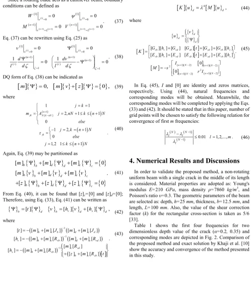
In order to validate the proposed method, a non-rotating uniform beam with a single crack in the middle of its length is considered. Material properties are adopted as: Young's modulus E=210 GPa, mass density ρ=7860 kg/m3, and [image:7.595.51.556.103.667.2]Poisson's ratio υ=0.3. The geometric parameters of the beam are selected as: depth, h=25 mm, thickness, b=12.5 mm, and length, L=100 mm. Also, the value of the shear correction factor (k) for the rectangular cross-section is taken as 5/6 [33].
Table 1. First four frequencies (Hz) of a uniform beam with a single crack in the middle of its length.
Exact solution[10] Proposed method
α
f4
f3
f2
f1
f4
f3
f2
f1
35888.7 22962.3
9393.7 1948.2
35944.39 22966.48
9411.22 1949.46
0.2
34219.7 22803.8
8350.7 1856.8
34312.69 22812.42
8399.43 1862.01
0.35
Difference (%)
f4
f3
f2
f1
0.155174 0.018204
0.186508 0.064675
0.271744 0.037801
[image:8.595.82.532.98.519.2]0.583544 0.28059
Table 2. Fundamental frequency of a rotating uniform blade.
2
γ 0 1 2 3 4 5 10
2 1
λ
Proposed method 3.482617 3.646401 4.063282 4.698882 5.534893 6.395305 11.04604
Kaya, 2006 [28] 3.4798 3.6445 4.0971 4.7516 5.5314 6.3858 11.0643
[image:8.595.95.515.554.716.2]Difference (%) 0.0810 0.0522 -0.8254 -1.1095 0.0631 0.1488 -0.1650
Figure 2. First four modes of a non-rotating uniform beam with an open crack in the middle of its length.
0 0.2 0.4 0.6 0.8 1
-1 -0.8 -0.6 -0.4 -0.2 0 0.2 0.4 0.6 0.8 1
ξ
v
α = 0.2
0 0.2 0.4 0.6 0.8 1
-1 -0.8 -0.6 -0.4 -0.2 0 0.2 0.4 0.6 0.8 1
ζ
v
α = 0.35
0 0.5 1 1.5 2
2 2.1 2.2 2.3 2.4 2.5 2.6 2.7 2.8 2.9 3
γ
λ 1
δ=0
δ=0.1
δ=0.5
δ=1
δ=2
0 0.5 1 1.5 2
4.2 4.4 4.6 4.8 5 5.2 5.4 5.6
γ
λ 2
δ=0
δ=0.1
δ=0.5
δ=1
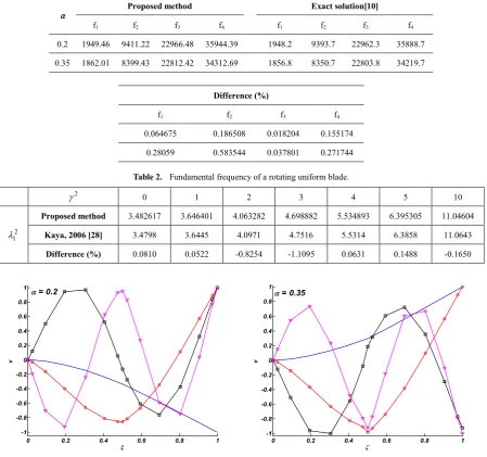
Figure 3. First four frequencies of a conical blade versus the angular velocity for various values of the hub radius
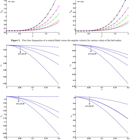
Figure 4. First four frequencies of a uniform blade versus the intensity of crack for various numbers of cracks
Consider an intact uniform rotating blade with r=1/30, E/kG=3.059, and δ=0. Values of the fundamental frequencies are presented in Table 2 for different values of the angular velocity of spin. The versatility of the proposed technique is confirmed by comparison of obtained results with the results of exact solution presented by Kaya [28].
Also, a conical blade with r=0.03, s=0.05 is considered that diameter varies as d=d0(1-0.5ξ). Fig. 3 shows the values
of the lowest four frequencies versus the value of the angular velocity for different values of the hub radius. As shown in this figure, values of the all frequencies increase as the value
of the angular velocity and hub radius increase. This is due to increasing of centrifugal force for higher values of angular velocity and hub radius.
Consider a uniform blade (r=0.03, s=0.05, h/L=0.1, δ=0.4, γ=1) with equally spaced similar open cracks. Fig. 4 shows the values of the first three dimensionless frequencies versus intensity of crack for various numbers of open cracks. As shown in this figure, because of the reduction in the stiffness of the beam, as numbers and depth of the cracks increase, all frequencies decrease.
0 0.5 1 1.5 2
6.6 6.7 6.8 6.9 7 7.1 7.2 7.3 7.4 7.5 7.6
γ
λ3
δ=0
δ=0.1
δ=0.5
δ=1
δ=2
0 0.5 1 1.5 2
9 9.1 9.2 9.3 9.4 9.5 9.6 9.7 9.8 9.9
γ
λ4
δ=0
δ=0.1
δ=0.5
δ=1
δ=2
0 0.05 0.1 0.15 0.2
1.82 1.84 1.86 1.88 1.9 1.92
α
λ1
n=1,3,5,10
0 0.05 0.1 0.15 0.2
4.25 4.3 4.35 4.4 4.45 4.5 4.55 4.6
α
λ2
n=1,3,5,10
0 0.05 0.1 0.15 0.2
6.9 6.95 7 7.05 7.1 7.15 7.2 7.25 7.3 7.35 7.4
α
λ3
n=1,3,5,10
0 0.05 0.1 0.15 0.2
9.3 9.4 9.5 9.6 9.7 9.8 9.9 10
α
λ4
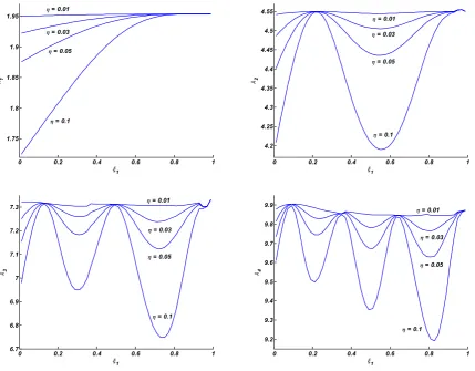
[image:9.595.84.518.111.577.2]Figure 5. First four frequencies of a wedge blade versus the position of a single crack for various values of intensity of crack A truncated wedge blade (r=0.03, s=0.05, δ=0.05, γ=1) is
considered with the width and depth of b=b0(1-0.1ξ) and
h=h0(1-0.1ξ) where h0=0.5L, respectively. Consider a single
crack with a constant depth as ac=ηh0 in a desired position on
the blade. Fig. 5 shows the variation of the first four frequencies versus the position of the crack for various values of η. It can be concluded that the effect of the crack has its highest effect on a natural frequency, when the crack is located at a point which has maximum value of curvature in the corresponding normal mode; for example clamped end for first mode. Reversely, it has little effect on a natural frequency when the crack is located at the inflection point of the corresponding normal mode like the free end for all modes. It should be noticed that as this figure reveals, numbers of these points increase in higher modes.
5. Conclusions
DQEM analysis of free transverse vibration of a rotating non-uniform Timoshenko blade with multiple open cracks was presented. Comparison of the proposed method with the exact solutions available in the literature revealed the excellent accuracy of this method. Also, effects of location, depth, and numbers of cracks as well as the angular velocity
of the spin are investigated on the natural frequency of the blade. The results showed that existence of cracks in the blade decrease the frequencies. Also, increasing the numbers of the cracks and the crack depth reduce the natural frequencies. It can be concluded that the damage has the highest effect on a natural frequency when the crack is located at a point which has maximum value of curvature in the corresponding normal mode. Reversely, it has little effect on a natural frequency when the crack is located at inflection point of the corresponding normal mode. Numerical results also showed that all natural frequencies increase when angular velocity of spin increases.
REFERENCES
[1] S. Caddemi, A. Morassi. Crack detection in elastic beams by
static measurements, International Journal of Solids and Structures, Vol. 44, 5301-5315, 2007.
[2] A. Morassi. Crack induced changes in eigenfrequencies of
beam structures, Journal of Engineering Mechanics, Vol. 119, 1798-1803, 1993.
[3] A. Morassi. Identification of a crack in a rod based on
changes in a pair of natural frequencies, Journal of Sound and
0 0.2 0.4 0.6 0.8 1
1.75 1.8 1.85 1.9
1.95 η = 0.01
η = 0.03
η = 0.05
η = 0.1
ξ1
λ1
0 0.2 0.4 0.6 0.8 1
4.2 4.25 4.3 4.35 4.4 4.45 4.5 4.55
η = 0.01
η = 0.03
η = 0.05
η = 0.1
ξ1
λ2
0 0.2 0.4 0.6 0.8 1
6.7 6.8 6.9 7 7.1 7.2
7.3 η = 0.01
η = 0.03
η = 0.05
η = 0.1
ξ1
λ3
0 0.2 0.4 0.6 0.8 1
9.2 9.3 9.4 9.5 9.6 9.7 9.8
9.9 η
= 0.01
η = 0.03
η = 0.05
η = 0.1
ξ1
Vibration, Vol. 242, 577-596, 2001.
[4] Y. Narkis. Identification of crack location in vibrating simply supported beams, Journal of Sound and Vibration, Vol. 172, 549-558, 1994.
[5] S.A. Paipetis, A.D. Dimarogonas. Analytical Methods in
Rotor Dynamics, Elsevier Applied Science, London, 1986.
[6] P.F. Rizos, N. Aspragathos, A.D. Dimarogonas.
Identification of crack location and magnitude in a cantilever beam from the vibration modes, Journal of Sound and Vibration, Vol. 138, 381-388, 1990.
[7] D.Y. Zheng, S.C. Fan. Natural frequency changes of a
cracked Timoshenko beam by modified Fourier series, Journal of Sound and Vibration, Vol. 246, 297-317, 2001.
[8] S.P. Lele, S.K. Maiti. Modeling of transverse vibration of
short beams for crack detection and measurement of crack extension, Journal of Sound and Vibration, Vol. 257, 559-583, 2002.
[9] H.P. Lin. Direct and inverse methods on free vibration
analysis of simply supported beams with a crack, Engineering Structures, Vol. 26, 427-436, 2004.
[10] N. Khaji, M. Shafiei, M. Jalalpour. Closed-form solutions for crack detection problem of Timoshenko beams with various boundary conditions, International Journal of Mechanical Sciences, Vol. 51, 667-681, 2009.
[11] M. Krawczuk, M. Palacz, W. Ostachowicz. The dynamic
analysis of a cracked Timoshenko beam by the spectral element method, journal of Sound and Vibration, Vol. 264, 1139-1153, 2003.
[12] J.A. Loya, L. Rubio, J. Fernandez-Saez. Natural frequencies
for bending vibrations of Timoshenko cracked beams, Journal of Sound and Vibration, Vol. 290, 640-653, 2006.
[13] R. Bellman, B.G. Kashef, J. Casti, Differential quadrature: A technique for the rapid solution of nonlinear partial differential equations, Journal of Computational Physics, Vol. 10, 40-52, 1972.
[14] R. Bellman, R.S. Roth, System identification with partial
information, Journal of Mathematical Analysis and applications, Vol. 68, 321-333, 1979.
[15] C.W. Bert, S.K. Jang, A.G. Striz, Two new approximate
methods for analyzing free vibration of structural components, AIAA Journal, Vol. 26, 612-618, 1988.
[16] C.W. Bert, M. Malik, Free vibration analysis of tapered
rectangular plates by differential quadrature methods: A semi-analytical approach, Journal of Sound and Vibration, Vol. 190, 41-63, 1996.
[17] C.W. Bert, M. Malik, The differential quadrature method for
irregular domains and application to plate vibration, International Journal of Mechanical Sciences, Vol. 38, 589-606, 1996.
[18] C.W. Bert, M. Malik, Differential quadrature method in
computational mechanics: A review, Applied Mechanics Reviews, Vol. 49, 1-28, 1996.
[19] C.W. Bert, X. Wang, A.G. Striz, Differential quadrature for
static and free vibration analysis of anisotropic plates, International Journal of Solids Structures, Vol. 30, 1737-1744,
1993.
[20] C.W. Bert, X. Wang, A.G. Striz, Convergence of the DQ
method in the analysis of anisotropic plates, Journal of Sound and Vibration, Vol. 170, 140-144, 1994.
[21] C.N. Chen. Vibration of non-uniform shear deformable
axisymmetric orthotropic circular plates solved by DQEM, Composite Structures, Vol. 53, 257-264, 2001.
[22] C.N. Chen. DQEM vibration analyses of non-prismatic shear
deformable beams resting on elastic foundations, Journal of Sound and Vibration, Vol. 255, 989-999, 2002.
[23] C.N. Chen. DQEM analysis of in-plane vibration of curved
beam structures, Advances in Engineering Software, Vol. 36, 412-424, 2005.
[24] C.N. Chen. DQEM analysis of out-of-plane vibration of
non-prismatic curved beam structures considering the effect of shear deformation, Advances in Engineering Software, Vol. 39, 466-472, 2008.
[25] P. Malekzadeh, G. Karami, M. Farid. A semi-analytical
DQEM for free vibration analysis of thick plates with two opposite edges simply supported, Computer Methods in Applied Mechanics and Engineering, Vol. 193, 4781-4796, 2004.
[26] K. Torabi, H. Afshari, M. Heidari-Rarani. Free vibration
analysis of a non-uniform cantilever Timoshenko beam with multiple concentrated masses using DQEM, Engineering Solid Mechanics, Vol. 1, 9-20, 2013.
[27] K. Torabi, H. Afshari, F. Haji Aboutalebi. A DQEM for
transverse vibration analysis of multiple cracked non-uniform Timoshenko beams with general boundary conditions, Computers and Mathematics with Applications Vol. 67, 527-541, 2014.
[28] M.O. Kaya. Free vibration analysis of a rotating Timoshenko
beam by differential transform method. Aircraft Engineering and Aerospace Technology, Vol. 78, 194-203, 2006
[29] H. Du, M.K. Lim, N.R. Lin. Application of generalized
differential quadrature method to structural problems, International Journal for Numerical Methods in Engineering, Vol. 37, 1881-1896, 1994.
[30] H. Du, M.K. Lim, N.R. Lin. Application of generalized
differential quadrature to vibration analysis, Journal of Sound and Vibration, Vol. 181, 279-293, 1995.
[31] R.M. Lin, M.K. Lim, H. Du. Deflection of plates with
nonlinear boundary supports using generalized differential quadrature, Computer and Structures, Vol. 53, 993-999, 1994.
[32] G. Karami, P. Malekzadeh. A new differential quadrature
methodology for beam analysis and the associated differential quadrature element method, Computer Methods in Applied Mechanics and Engineerig, Vol. 191, 3509-3526, 2002.
[33] S. Timoshenko, D.H. Young, W. Weaver. Vibration
Problems In Engineering, Wiley, New York, 1974.
[34] H. Tada, P. Paris, G. Irwin. The Stress Analysis of Cracks
Handbook, Paris Productions, St. Louis, 1985.
[35] A. Valiente, M. Elices, F. Ustaris. Determinacion de