Designing of Automotive Engine Electronic Throttle
Controller for EF7 Engine
Mehdi Rostami, Parviz Amiri
*Shahid Rajaee Teacher Training University, Iran, Tehran *Corresponding Author: [email protected]
Copyright © 2014 Horizon Research Publishing All rights reserved.
Abstract
In the new Automotives Engines ElectronicThrottle has been used to reduce fuel consumption and increase the torque. The throttle’s butterfly valve angle is changed by Engine Control Unit (ECU) Signals. In some cases physical model of Electronic Throttle is needed for engine optimization in automotive industrial. In this paper physical parameters of the special engine electronic thottle has been gotten and estimated. After this research, a controller has been designed and constructed. Software simulation results show the controller works correctly.
Keywords
Engine Electronic Throttle, Physical Model,Parameter Estimation, Controller
1. Introduction
In many circumstances, the car does not need to use the maximum engine power. Therefore torque and power output must be controlled. It is the duty of the throttle valve in internal combustion engines. This instrument controls the amount of input air to engine by butterfly valve then fuel injection will diminish and torque and power grows [1]. Usual throttle valves are controlled by 2 mechanisms: 1- Mechanical Throttle 2- Electronic Throttle. In this paper we will research on Electronic Throttle. In Electronic Throttle, ECU controls butterfly valve’s angle. This instrument consists of 5 parts : DC motor , butterfly valve, spring , gears and potentiometer. For accurate controlling of this type of throttle, physical model must be recognized. In this research at first a physical model has been yield by mechanical equations then for recognizing of unknown parameters, estimation method was used [2-4].
2. Materials and Methods
Process of this portion consists of 4 steps. They are primary physical model, experiment, estimation and evaluation.
2.1. Throttle Physical Model
For recognizing of physical model the throttle is divided to 2 parts: 1- DC Motor 2- Mechanical Model. In continues we will interpret these parts.
2.1.1. DC Motor
[image:1.595.361.505.350.426.2]Model of DC Motor consists of a resistor, inductor and non electromotive voltage [2, 3]. In figure 1 these parts has been demonstrated.
Figure 1. Electrical model for DC Motor
Equations 1 and 2 annotate electrical and mechanical mechanism of DC motor.
(1)
)
(
)
(
t
K
i
t
T
=
t×
(2)In above equations Ra is armature resistance, La is coil inductance, Kt is electromechanical constant and T(t) is output engine torque. For modeling of DC motor must be notice figure 2.
Figure 2. Curves of current and torque
These curves (in figure 2) illustrate 2 notes. In current curve inductor produces delay in system and in torque curve the torque is proportional with current [5]. From those notes,
) ( ) ( )
( . )
( v t
dt t di L t i R t
[image:1.595.323.544.573.705.2]the DC motor mechanism is summarized to equation 3 and figure 3.
) ( )
(t Kt U t td
[image:2.595.327.542.193.340.2]T = × − (3)
Figure 3. Final DC Motor model 2.1.2. Mechanical body
For modeling the mechanical body should be notice 3 parameters they are: butterfly inertia (J), friction of butterfly and body (c) and spring constant (k) [5].These parameters relates corresponding with equation 4.
(4) In 4 T is DC motor torque and Ө is butterfly angle. In throttle body for abatement of 360 degrees rotation of butterfly, 2 barriers have been produced in body. They are in 15 degrees and 90 degrees position. The 15 degree position is named limp home zone. The limp home zone produces a nonlinearity effect in system. The body torque effect in 4 is a torque that is named Tb (relation 5):
(5) Tb in 5 is defined by 6:
(6)
[image:2.595.95.265.489.601.2]The G coefficient in 5 will be known in continues. The simulink model of Tb is demonstrated in figure 4.
Figure 4. The simulink model of Tb
In the figure 6 model parameters have been defined in table 1:
Table 1. Parameters amounts of figure 6
Parameter Name Definition Amount H Maximum Zone 1.57rad =90 degree L Minimum Zone
0.26 rad= 15 degree
G Torque Gain ---X Input(angle) ---F Output(Torque)
---Now the Laplace conversion of relation 6 is relation 7:
)
(
)
(
)
(
))
0(
)
(
(
))
0(
)0
(
)
(
(
2s
T
s
T
s
k
s
s
c
s
s
s
J
b+
=
+
−
+
′
−
−
θ
θ
θ
θ
θ
θ
(7)
The primary states of the relation 7 is 8:
(8) By the relation 7 we will get the simulink model that has been demonstrated in figure 5:
Figure 5. Simulink Model of relation 7
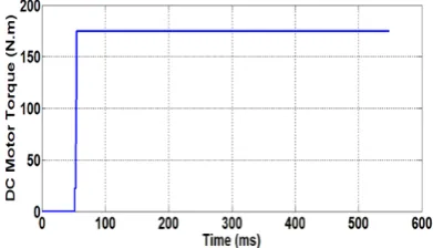
In figure 5 at first the T torque enters to system then mixes by returned signals, they are c (Damping of friction) and k (spring constant) and Tb. The Tb appears in ends of butterfly path. The input of model is demonstrates in figure 6.The returned signals has been demonstrated in figure 7,In figure curve 7 the spring torque has grown linearly because the spring has been compressed and the friction is constant approximately. In figure 8 against torque Tb has appeared in 90 degrees zone hence in time 380ms some vibrations have been produced.
Figure 6. Torquesignal curve from DC motor
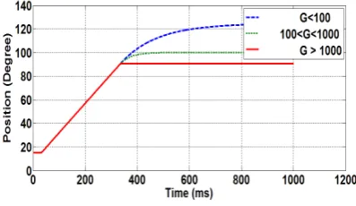
The resultant inertia signal has been demonstrated in figure. In figure 9 at the Limp Home zone inertia is positive and in maximum of zone the inertia is positive and negative because of some vibrations. The velocity signal in this model has been demonstrated in figure 10. In this figure the velocity is fixed in time of butterfly’s rotation but it has some vibrations in time 380 ms because of contacting by body. The positions of butterfly has been demonstrated in figure 11, for G>1000 the curve is best than other of G ranges. The gotten model in figure 5 is a general model for many types of
T
k
c
J
θ
..+
θ
.+
θ
=
b
T
T
k
c
[image:2.595.334.530.497.609.2]throttle body. If this model would be for a special throttle body the parameters value c, J, k, kt and td would be
[image:3.595.332.531.78.193.2]recognized. In continues we will get parameters value of Bosch Electronic throttle body.
[image:3.595.73.285.132.257.2]Figure 7. Spring torque and Friction torque
[image:3.595.60.294.194.708.2]Figure 8. Hard Stop output signal
Figure 9. Resultant inertia signal
Figure 10. velocity signal of butterfly
Figure 11. Butterfly location in time
2.2. Getting of Data from Experiment
In this section the step response of electronic throttle body of Bosch company that has type number (0 280 750 257) has been gotten (This type of electronic throttle has been used in Iran Khodro Company for EF7 National Engine). The experiment set in this process has 2 sections of software and hardware. The hardware part consists of throttle body, Data Acquisition Card and PC. The butterfly position has been measured by TPS 1 and transmitted to PC. The yielded data
from this experiment after filtration has been demonstrated in figure 12.
Figure12. TPS data after filtration
2.3. Getting the Unknown Parameters
For getting of the unknown parameters has been compared physical model and experiment result [6]. In this method the estimation tool in MATLAB software has been used. The unknown parameters have been found by this method. The measured and estimated curves have matched approximately in figure 13 but the maximum errors exist in time of 140ms to 250ms. The error curve has been demonstrated in figure 14. The unknown parameters have been gotten in 77 iteration processes in MATLAB tool and have been listed in table 2.
Table2. The unknown parameters value Dimension Value
Parameter
N.m/A 246.4
kt
S 0.01
td(Input_delay)
N.m/rad 23.5
K
N.m 0.32
J
N.m.s/rad 12.6
C
1-Throttle Position Sensor
[image:3.595.65.290.291.545.2] [image:3.595.329.535.369.481.2]Figure 13. The estimated and measured curves
Figure 14. The error curve between estimated and measured curve
2.4. The Controller Designing for Physical Model
Now must be design a controller for the physical model that is changed following of automotive throttle pedal. This controller is one of the ECU circuits. The parts of this controller have been demonstrated in figure 15. In the controller at first car driver pushes the pedal then the pedal signal is transmitted to ECU. The pedal signal is as reference signal. In the ECU throttle butterfly angle signal and reference signal have been compared in comparator portion and the error signal is produced. Then the error signal has been sent to DC motor driver. The driver portion acts by PWM2 method. The duty cycle of PWM signal is dependent
to error signal. The higher error leads to higher duty cycle and vice versa. Also in this method, the butterfly direction is changed by getting of positive and negative voltage (as PWM). So two important portion of this controller is comparator and motor driver. In continues we will explain these two portions [7-9].
Figure 15. The controller parts
2-Pulse Width Modulation
A. Comparator portion:
The portion consists of 2 comparators. Comparators inputs are symmetry and then output signals are and by PWM signal. In continues output PWM signal multiply to positive or negative gain because we need positive or negative voltage for DC motor direction. The figure 16 has demonstrated the comparator portion.
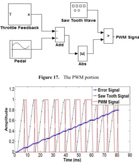
Figure 16. The comparator portion B. PWM portion:
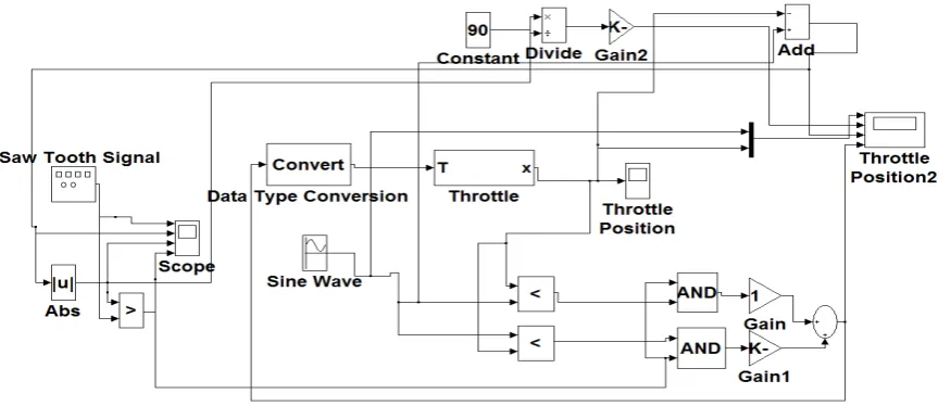
The PWM method has been used to control of the motor speed. To producing of PWM signal the error magnitude and a saw tooth wave are compared.The frequency of saw tooth signal is 25 kHz. The portion has been demonstrated in figure 17. Figure 18 demonstrates PWM, error and saw tooth curves. The complete model of controller has been demonstrated in figure 19. The 2 important portions exist in the figure.
Figure 17. The PWM portion
Figure 18. PWM, error and saw tooth curves
[image:4.595.72.284.70.376.2] [image:4.595.320.548.166.288.2] [image:4.595.318.549.429.700.2] [image:4.595.78.277.639.717.2]Figure 19. The complete controller diagram.
2.5. The Software Simulation Results
Now a reference signal as pedal signal (see figure 20) is exerted on controller then the butterfly position has been demonstrated in figure 21. In figure 21 some vibrations has been existed in up and down border sides. In figure 22 we accommodated the curves of figures 20 and 21 and in figure 23 the error signal between those signals has been demonstrated. The maximum errors in the error signal are 7 percents. These errors appear in limp home zone mostly.
Figure 20. The reference signal
Figure 21. The butterfly position
[image:5.595.90.528.75.262.2]Figure 22. Accomodation of before signals(figure 20&21)
Figure 23. Error signal
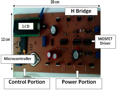
2.6. The Construction of Controller Circuit
The controller circuit consists of 2 portions. They are controller and driver portions. The controller portion can be Microcontroller or FPGA. In the structures that have many inputs and outputs, FPGA is useful but in this structure Microcontroller is enough [6, 10, 11]. The structure has been demonstrated in figure 24.
[image:5.595.329.537.295.440.2] [image:5.595.68.291.413.730.2] [image:5.595.328.534.414.598.2]to DC motor driving. In the bipolar chopper portion, the H bridge structure has been used [12, 13]. The maximum current of driver portion is gotten Ohm law. The coil resistance of throttle is 1.6 ohms and the voltage supply is 12 volts then the consuming current is:
Figure 24. The controller structure by Microcontroller [6] The H Bridge of this circuit consists of MOSFET IRF3205 and driver ICs IR2110. The freewheeling diodes (1N5818 Schottky diodes) have been used to protection of transistors from returned currents. The mechanism of this controller has been explained in flowchart of figure 25.
The designed circuit of the driver portion has been demonstrated in figure 26. In this circuit the IR2110 ICs are MOSFET driver. The constructed circuit has been demonstrated in figure 27. In the constructed circuit the H
bridge circuit lines would be thick because of high current crossing. This circuit has been used in an experiment set. In this experiment a pulse signal that is 5 Hz has exerted as pedal signal to microcontroller. The microcontroller receives the throttle’s potentiometer signal too. By comparing of the signals and producing of proper PWM signal, the throttle motor is controlled. The maximum error of these curves is 8.
Error= (9)
Figure 25. The controller’s flowchart
Figure 26. The circuit of driver portion
A
I
=
12
/
1
.
6
=
7
.
5
% 8 100 5
4 . 0
100= × = ×
MAX Error
[image:6.595.70.290.145.302.2] [image:6.595.330.551.170.379.2] [image:6.595.98.528.457.640.2]Figure 27. The controller circuit
3. Conclusion
In this paper a physical model of special ETC has been approximated and then designed and constructed a controller for it. The maximum error of this controller in software simulation is 7 percents and maximum error in experiment set is 8 percents. Errors between Simulation results and lablatory results are 1 percent and this subject shows the controller works correctly.
REFERENCES
[1] Jeffrey A. Cook, Fellow IEEE, Ilya V. Kolmanovsky, Senior Member IEEE ,”Control, Computing and Communications: Technologies for the Twenty-First Century Model T”, Proceedings of the IEEE | Vol. 95, No. 2, February 2007 [2] Jansri, A,” On practical control of electronic throttle body”,
Industrial Electronics Society, IECON. 30th Annual Conference of IEEE,2004
[3] Guvenc, L.; Uygan, I. M. C.; Kahraman, K.; Karaahmetoglu, “Cooperative Adaptive Cruise Control Implementation of Team Mekar at the Grand Cooperative Driving Challenge”, Intelligent Transportation Systems, IEEE Transactions on Volume: 13, April 2012
[4] Toshihiro Aono and Takehiko Kowatari, “Throttle-Control Algorithm for Improving Engine Response Based on Air-Intake Model and Throttle-Response Model”, IEEE TRANSACTIONS ON INDUSTRIAL ELECTRONICS, VOL. 53, NO. 3, JUNE 2006
[5] Johan Gagner Rickard Bondesson,” Adaptive Realtime Control of a Nonlinear Throttle Unit “, master of science thesis in Automatic Control , Lund Institute of Technology,February 2000
[6] Xiaofang Yuan and Yaonan Wang , “A Novel Electronic-Throttle-Valve Controller Based on approximate Model Method “ , IEEE TRANSACTIONS ON INDUSTRIAL ELECTRONICS, VOL. 56, NO. 3, MARCH 2009
[7] Vasak, M, “Electronic throttle state estimation and hybrid theory based optimal control”, Industrial Electronics, IEEE International Symposium , May 2004
[8] Okuyama, Y, “PID control for nonlinear discretized systems “,SICE, Annual Conference Sept. 2007
[9] Liu, Jiang ,Study on electronic throttle system controller design , Vehicular Electronics and Safety (ICVES), IEEE International Conference ,July 2010
[10] Qian Weikang , “Practical solution for automotive electronic throttle control based on FPGA”, Signal Processing, ICSP. 9th International Conference Oct. 2008
[11] Loh, R.N.K ,”Modeling, parameters identification, and control of an electronic throttle control (ETC) system”, Intelligent and Advanced Systems,.ICIAS . International Conference ,Nov. 2007
[12] Qiang Li, ”The study of PWM methods in permanent magnet brushless DC motor speed control system”, Electrical Machines and Systems,. ICEMS. International Conference , Oct. 2008
[image:7.595.183.429.77.272.2]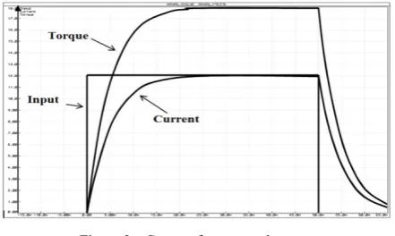
![Figure 24. The controller structure by Microcontroller [6]](https://thumb-us.123doks.com/thumbv2/123dok_us/8755383.892767/6.595.98.528.457.640/figure-controller-structure-microcontroller.webp)