Minimizing engine emissions using state feedback control with LQR and artificial intelligence fuel estimator

Citation:

Chan, KY and Ordys, A and Duran, O and Volvov, K and Deng, J (2014) Minimizing engine emissions using state-feedback control with LQR and artificial intelligence fuel estimator. International Journal of Innovative Research in Science, Engineering and Technology, 2 (3). pp. 1-9. ISSN 2319-8753

Link to Leeds Beckett Repository record: http://eprints.leedsbeckett.ac.uk/4336/

Document Version: Article

Creative Commons: Attribution 4.0

The aim of the Leeds Beckett Repository is to provide open access to our research, as required by funder policies and permitted by publishers and copyright law.

The Leeds Beckett repository holds a wide range of publications, each of which has been checked for copyright and the relevant embargo period has been applied by the Research Services team.

We operate on a standard take-down policy. If you are the author or publisher of an output and you would like it removed from the repository, please contact us and we will investigate on a case-by-case basis.

International Journal of Innovative Research in Technology & Science(IJIRTS)

1 Minimizing Engine Emissions using State-feedback Control with LQR and Artificial Intelligence Fuel Estimator

Minimizing Engine Emissions using State-feedback

Control with LQR and Artificial Intelligence Fuel

Estimator

K.Y. Chan, Prof. A. Ordys, Senior Member, IEEE, Dr. O. Duran, Member, IEEE, and Dr. K. Volkov, Member, MIMechE Dr. J. Deng, Senior Member, IEEE

Abstract

This paper presents a novel engine controller targeting the reduction of gas emissions. Toxic emissions, such as Carbon Monoxide (CO) and Nitric Oxide (NOx) affect the environment and the authorities aim to limit their amount by law. Emissions are formed during the high temperature combustion process, and can be optimised by adjusting some engine operating parameters. In this paper, the model describing emissions output of the engine as a function of engine control parameters is represented as a state-space system. A closed-loop controller is developed by using state-feedback control algorithm. The closed-loop gain, K, is obtained from the LQR tuning principles. The fuel estimator developed in previous works is used in order to reduce the model from the 8th order. The results show that the controller is able to control emission to the minimum in all constraints while keeping engine running in the same performance.

I.

Introduction

Engine combustion performance can be affected by engine operating parameters, such as fuel to air ratio, ignition timing, and the valve opening and closing event [13], hence emission control can be achieved by system identification of an inverse engine combustion process and optimisation using closed-loop control algorithms. To achieve this, various sensors are fitted onto the engine in order to monitor the combustion process. They are able to collect exhaust gas information, including the amount of carbon dioxide (CO2), oxygen (O2), carbon monoxide (CO) and nitric oxide (NOx), as well as the condition of exhaust gas including exhaust gas temperature and pressure [7]. The Engine Control Unit (E.C.U.) can use such information to calculate the optimal engine operating parameters to control the emissions while keeping the engine in the best possible performance. The exhaust substance contains CO and NO, which are considered as pollutants and the maximum amount allowed is regulated by law.

The other area that works in minimizing emissions focuses on the fuel composition research. Gas exchange

process is summarized next. The atmosphere air contains Nitrogen (N) and Oxygen (O) while fuel contains Hydrogen (H) and Carbon (C) atoms. Products are formed in the combination of C, H, O and N during the high temperature engine combustion process. The main toxic by-products discovered are CO and NOx. Fuels are usually a blend of gasoline with a type of alcohol, such as methanol and ethanol, to reduce toxic emissions. However further engine control is needed in order to understand the correct composition of fuel injected into engine. Pioneering in that direction, artificial intelligence has been successfully proposed [3][4].

In this paper, an emission controller is developed. The controller is tested using engine simulations based on 1st law of thermodynamic [ref to our paper in the model development]. The engine simulation is able to generate the exhaust gas composition and allow off-line research on control algorithms [14]. This paper is organised as follows. The methodology of the paper is discussed in Section II. The development of the artificial intelligence fuel estimator is discussed in Section III. The SI engine and representation of the space model is discussed in Section IV. The state-feedback model and its results are analysed in Section V. Finally conclusions are drawn in Section VI.

II.

Methodology

Engine simulation is used in this paper instead of engine test bed. The main advantages for using engine simulation are the flexibility and low-cost. In real engine development, such research may require heavy demand of mechanical systems or even engine modifications which usually are not cost-effective on commercial engines. For example, in mechanical Variable Valve Timing (VVT) systems, it is required to fit a large mechanical system onto the intake manifold. Another example is a cylinder pressure sensor that would require drilling holes for its installation into the cylinder.

ISSN:2321-1156

International Journal of Innovative Research in Technology & Science(IJIRTS)

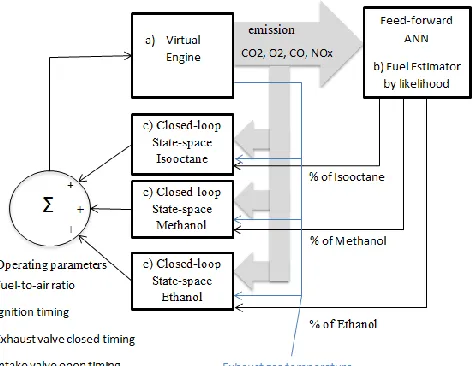
closed-loop state-space controller. Figure 1 presents the block diagram of the engine control. The engine parameters, including fuel to air ratio, ignition timing, exhaust valve closed timing and intake valve open timing, are used as the input parameters to control the level of emission in the virtual engine. The reason for choosing those parameters are explained in early studies [3][4]. The controller estimates the original fuel composition using artificial neural network. The fuel estimator is able to find the probability distribution of the likelihood of the given fuels. This provides the proportional control to the state-feedback controller according to the fuel composition.

Figure 1 Block diagram of the engine control algorithm

A.

Air and Fuel Properties

Engines take air from the atmosphere and work with fuels with different fuel compositions provided by the suppliers. Dry air consists of mainly 79% of nitrogen and 21% of oxygen. A more detailed composition of dry air is shown in Table 1.

Table 1 Principle constituents of dry air [11]

Gas ppm by volume

Molecular weight

Mole fraction

Molar ratio Oxygen 209500 31.998 0.2095 1 Nitrogen 780900 28.012 0.7905 3.773

Argon 9300 38.948 NIL NIL Carbon

dioxide

300 40.009 NIL NIL

Air 1000000 28.962 1.000 4.773

Fuel suppliers provide a blended composition with alcohol which includes small amounts of oxygen atoms, to help with the reduction of CO in the emissions. Therefore, three

commonly used fuel compositions are considered here, including Isooctane, Methanol and Ethanol.

Table 2 Fuel compositions being tested according to [6], [11], and [16]

Fuel # of C atoms

#of H atoms

# of O atoms

Chemical symbol

Isooctane_r [16] 8 18 0 C8-H18

Isooctane_h [11] 8 18 0 C8-H18

Methanol_f [6] 1 4 1 C1-H4-O1

Methanol_h [11] 1 4 1 C1-H4-O1

Ethanol_h [11] 2 6 1 C2-H6-O1

B.

Virtual Engine

The- test run is based on a virtual 4-stokes spark-ignition (SI) engine. Recent works have been done on the estimation of the four strokes engine [2]. They are involved in different engine processes, including volumetric efficiency, heat transfer and gas exchange. Heat release calculation is only generated in combustion stroke. The engine pressure is calculated in a single zone, and temperature is calculated in two zones, burned and unburned zone. The unburned zone is used prior to the combustion process without any heat being generated during combustion. The burned zone calculates the temperature with heat release estimation. The work done is calculated by volume from the crank-slider model. The burning process and heat transfer are calculated by using sub-models as shown in Table 3.

Table 3 Sub-models use in engine simulation modelling

Process Sub-models

Work done Crank-slider model

Heat release in combustion Single Wiebe function

Heat transfer correlation Woschni function

Injection Port injection

Gas Exchange Thermal equilibrium

C.

Engine Data Collection

3 Minimizing Engine Emissions using State-feedback Control with LQR and Artificial Intelligence Fuel Estimator

emissions of three different fuels, which are Isooctane, Methane and Ethanol. The dataset contains 10500 samples, 3500 samples for each fuel. The training process used 60% of the data for training and 40% of data for network validation. When collecting the data, the engine runs at 2000rpm with a fixed torque. The dataset also records the behaviours of engine using random engine operating parameters, including fuel-to-air ratio, ignition timing and valves event. The ranges of these parameters are shown in Table 4. The contents of emission compositions recorded are CO2, O2, CO and NOx.

Table 4 Parameters and the ranges are used to record the experimental simulation dataset

Parameters Range

Fuel used Isooctane (C8H18)

Methanol (C1H4O1)

Ethanol (C2H6O1)

Fuel-to-air ratio 0.7 to 1.3 Ignition -10 to -40 deg Exhaust valve open timing 330 to 390 deg

Intake valve open timing 330 to 390 deg

III.

Fuel Estimator

Previous works have been done on estimating the actual fuel composition [3] [4]. The results prove the fuel estimator has a reasonable performance by using feed-forward artificial neural network. To provide the proportional control, the fuel estimator is needed to design the estimator of the likelihood of given fuel compositions. The transfer function used in the output layer is softmax. The ‘softmax’ transfer function returns a value between 0 and 1 according to Equation 1. The same dataset and training methods are applied for two different cases, namely Isooctane-Ethanol and Isooctane-Methanol.

Equation 1

A.

Case 1: Isooctane-Ethanol Mixture

The first case study is the estimation of probability using Isooctane-Ethanol mixture. The mixture contains Isooctane (C8H18) ranging between 70% to 100% and Ethanol (C2H6)

ranging between 0% to 30%, and one case with 100% Ethanol for reference of pure Ethanol. The results are presented in Table 5. The estimation of pure Isooctane is not accurate with the estimator returning 20% Ethanol for the pure 100% Isooctane case. . When the fuel contains a

portion of Ethanol, the neural network estimation is more accurate. The estimation of 100% Ethanol is very accurate, returning 98.76%. The neural network is able to provide further control to different portions of mixture of Isooctane-Ethanol.

Table 5 The probability of isooctane, methanol and ethanol estimated with isooctane- methanol mixture

Fuel Probability (%)

Isooctane Ethanol Isooctane Methanol Ethanol 100% 0% 80.45% 0% 19.55% 95% 5% 78.20% 0% 21.80% 90% 10% 75.86% 0% 24.14% 85% 15% 73.94% 0% 26.06% 80% 20% 72.37% 0% 27.63% 75% 25% 67.87% 0% 32.12% 70% 30% 66.80% 0% 33.20% 0% 100% 0.36% 0.88% 98.76%

B.

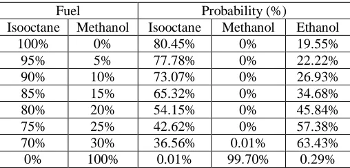
Case 2: Isooctane-Methanol Mixture

The second case is the estimation of probability for the mixture of Isooctane-Methanol mixture. The mixture contains Isooctane (C8H18) ranging between 70% to 100%

and Methanol (C1H4) ranging between 0% to 30%, and one

case with 100% Ethanol for reference. The results are presented in Table 6. The estimation of 100% Isooctane behaves as in Case 1. When the portion of Methanol is mixed with Isooctane, the estimator mistakenly identifies Ethanol instead of Methanol. This is due to the fact that the mixed compositions in terms of hydrocarbon are very similar. The estimation of 100% Methanol is 99.7% of. The neural network is developed for further control to different portion of mixture of Isooctane-Methanol.

Table 6 The probability of isooctane, methanol and ethanol estimated with isooctane- methanol mixture

Fuel Probability (%)

Isooctane Methanol Isooctane Methanol Ethanol 100% 0% 80.45% 0% 19.55% 95% 5% 77.78% 0% 22.22% 90% 10% 73.07% 0% 26.93% 85% 15% 65.32% 0% 34.68% 80% 20% 54.15% 0% 45.84% 75% 25% 42.62% 0% 57.38% 70% 30% 36.56% 0.01% 63.43% 0% 100% 0.01% 99.70% 0.29%

IV.

State-space Engine Model

ISSN:2321-1156

International Journal of Innovative Research in Technology & Science(IJIRTS)

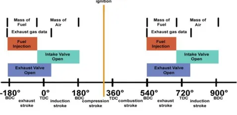
event due to division into strokes [9]. The engine operating parameters will not operate all the time throughout the engine event. A detailed diagram of the engine events and theirs’ operating parameters is presented in Figure 2. For example, the collection of exhaust gas information is valid while the exhaust gas valve is opened, and finishes while the valve is closed. The optimal ignition timing related to the past emissions information can be updated during to the time gap between the timing of exhaust valve closed and the igniting timing in the coming stroke.

Figure 2 The control event of a SI engine.

Engine emission is considered as non-linear behaviours [11][12]. To catch the dynamic of the engine emission against engine operating parameters, system identification method is needed [1][5][8][15]. The state-space representation is chosen to perform system identification. For real time system, the state-space equations are presented in Equation 2. The state-space is divided into two equations, the state equation and the measurement equation .

,

Equation 2

where

x is the state vector, u is the input vector, y is the output vector,

A is a n-by-n state weighting matrix, B is a n-by-m input weighting matrix, C is a l-by-n output weighting matrix,

D is a m-by-m back propagate weighting matrix, zero when there is no gain between input and output,

n is the number of state order, l is the number of outputs, m is the number of inputs.

Since the engine data is sampled, the state-space representation in discrete time is shown in Equation 3.

Equation 3

where,

the state vector is using the state value in the previous step, i.e. .

These four gains, A, B, C and D, can be estimated by the prediction error method (pem). Such method estimates the error of Nth order and finds the minimum cost by the following equations:-

Equation 4

The cost function, Vn(Ɵ,ZN), is used as in Equation 5 [8].

Equation 5

where,

Vn is the cost function

Zn is the measurement data

is the weighting matrix

eF(k,Ɵ) is the prediction error function and can be

determined by[8]:-

Equation 6

where,

L is the monic prefilter that can be used to enhance certain frequency regions.

G is process model H is white noise model

can be determined by the least squares method by minimizing the sum of the form of the output and the product of and the measurement data.

Equation 7

V.

State-feedback

Control

using

LQR

In order to design the closed-loop controller for state-space, the next step is to identify the state feedback control gain, K, which is in agreement with the state feedback control law shown in Equation 8.

u = -Kix,

Equation 8

where,

u is the output x is the input

5 Minimizing Engine Emissions using State-feedback Control with LQR and Artificial Intelligence Fuel Estimator

and state-space can be controlled as closed-loop system shows in by updating the input gain as

A-

Equation 9

where,

K is the closed-loop gain

Assume engine parameter is controllable against the emissions and engine performance/ Then the gain K can be obtained by using linear quadratic regulator (LQR) method which optimises the system at the minimum cost. The state-space can be optimised by a LQR with the minimum cost. LQR is calculated to minimize the cost function J(u). For a discrete engine system:-

Equation 10

where,

Q is the state cost, _,

R is the input cost, _and

N is the time horizon

The LQR can be solved by Riccati equation:-

Equation 11

The controller assumes the simplest case to control the system by choosing R = 1, and Q = C’.C. The cost function corresponding to Q and R share the equal importance in the state variables although this can be tuned.

Figure 3 Block diagram of closed-loop state-space system with closed-loop gain K obtained from LQR method

A.

State-feedback Control with Fuel

Estimator

In order to capture the engine behaviours covered the most of the situations, a large set of engine data is needed. The development of the state-space is hence generated the

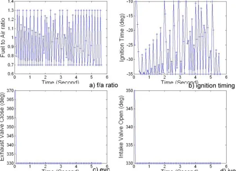
model with relatively higher order. The engine operating parameters of the 20th order state-space included all fuel comsition listed in Table 2 are presented in Figure 4. In this test the engine is running with pure Isooctane. Results showed that the state-space is unable to find the optimized engine operating parameters. For a) fuel to air ratio and b) ignition timing, the values are fluctuating between the maximum and minimum; and for c) exhaust valve closing timing and d) intake valve opening, the values are staying at the minimum. The model is unstable.

Figure 4 The optimised engine parameters in the 20th order state-space. a) is fuel-to-air ratio, b) is ignition timing is degree, c) is exhaust valve closed timing and d) is the intake valve opening timing

ISSN:2321-1156

International Journal of Innovative Research in Technology & Science(IJIRTS)

Figure 5 The optimised engine parameters in the 8th order state-space with fuel estimator. a) is fuel-to-air ratio, b) is ignition timing is degree, c) is exhaust valve closed timing and d) is the intake valve opening timing

B.

Controller test with Engine Cycle

Initial works in [2][3][4] performed test with a fixed set of parameters. By considerating the controller works under realistic condition, here, the engine cycle is introduced with the mapping of changes in speed. This allows to capture the behaviours of rapid and slow speed changes when the engine is accelerating or decelerating between 1000 rpm and 3000 rpm. The step of change is in every two seconds, allowing the engine controller to settle at the given speeds. The engine cycle used in the test is presented in Figure 6. It is noted that the tests are run on a fixed torque.

Figure 6 Engine cycle used in the final tests

To test that the developed engine control provides the optimisation of emissions, three engine simulations were performed, one with control and two without control, respectively... The engine cycle lasted 20 seconds. The engine parameters used without controller are fixed. The specifications of the engine run without control use two fuel-to-air ratios which are fixed at 0.95 and 1.05 respectively. The ignition timing is fixed at 25°. Exhaust valve closes at TDC (360°) and the intake valve opens at the same time. Two cases of Isooctane-Ethanol mixtures have been chosen for this comparison.

C.

Result with and without Controller

The levels of emissions found in species of CO2, O2, CO

and NOx with and without control are presented in Figure 7. The results show that when the engine has no control, the

levels of emissions are not at their minimum at all constraints. When the fuel to air ratio is 1.05 at leaner mixture (value over 1), the red lines in the graph show that the levels of CO2, O2 and NOx are at the lowest compared to

the other two results, but the level of CO is over 1%, thus exceeding the level allowed by legislation. Whereas when the fuel to air ratio is 0.95 at richer mixture, the black lines in the graph show the level of CO2 and CO are at

satisfactory levels. The negative effect is the level of NOx which is about eight times larger than the one resulting with control. Therefore it can be concluded that the controller identified optimal parameters in all level of emissions.

Figure 7 The level of emissions found in the engine simulation with and without control with given fuel-to-air ratio. a) is CO2,

b) is O2, c) is CO and d) is NOx

D.

Case 1: Isooctane-Ethanol Mixture

Case 1 tests the engine run with Isooctane-Ethanol mixture in the given engine cycle. The content of the mixture is similar to the test in Section IIIA, with the first test ran on 100% Isooctane. Four more tests are done with the mixture blended Ethanol into Isooctane by 10%, 20%, 30% and 40% respectively.

7 Minimizing Engine Emissions using State-feedback Control with LQR and Artificial Intelligence Fuel Estimator

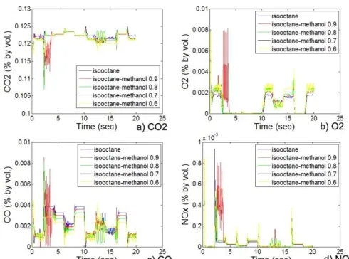
Figure 8 The level of emissions found in the engine control simulation of engine cycle in different portion of Isooctane-Methanol mixture. a) is CO2, b) is O2, c) is CO and d) is NOx

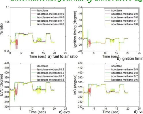
Figure 9 The engine operating parameters recorded in the engine control simulation of engine cycle in different portion of Isooctane-Methanol mixture. a) is fuel-to-air ratio, b) is ignition timing is degree, c) is exhaust valve closed timing and d) is the intake valve opening timing

E.

Case 2: Isooctane-Methanol Mixture

Case 2 test the engine run with Isooctane-Methanol mixture in the given engine cycle. The first test ran on 100% Isooctane. Four more tests are done with the mixture of blended Methanol into Isooctane by 10%, 20%, 30% and 40% respectively.

Figure 10 presents the level of emissions generated from the simulation with the given engine cycle. The related

engine operating parameters are presented in Figure 11. The results show that when the speed is changing, the controller settles quickly. It can be observed that when the speed varies, the emissions of CO2 and NOx have rapid increases

and CO decreases rapidly. The controller is able to settle the emissions quickly within a few engine revolutions.

One uncertainty found is in the result of 90% Isooctane and 10% of Methanol which is denoted by the red line. The controller has an unstable response between 2 to 4 seconds. The controller is unable to pick up the optimal engine operating parameters as shown in Figure 11 where the values of fuel to air ratio, ignition timing and valve events are fluctuating. The same trends happen at the results between 12 and 14 seconds. By analysing the speed at the moment where the uncertainties are found, we can note that they happen when the speed is increasing from 1000 rpm to higher speed. Therefore the controller performs worse at lower speed and the controller needs to improve by collecting more data while training the state-spaces. For the performance of the steady control, we can draw the same conclusion as in Case 1.

ISSN:2321-1156

International Journal of Innovative Research in Technology & Science(IJIRTS)

Figure 11 The engine operating parameters recorded in the engine control simulation of engine cycle in different portion of Isooctane-Methanol mixture. a) is fuel-to-air ratio, b) is ignition timing is degree, c) is exhaust valve closed timing and d) is the intake valve opening timing

VI.

Conclusions

This paper discusses the development of an engine controller which is able to optimise engine control parameters resulting in minimum levels of gas emissions while keeping the optimal performance in various speeds. Five input variables taken from the condition of exhaust gas have been identified, including the level of CO2, O2, CO and NOx in addition to the exhaust gas temperature. We are aiming to control four engine operating parameters, including fuel-to-air ratio, ignition timing, exhaust valve closed timing and intake valve opening timing.

Three fuel mixtures have been used for this investigation, including 100% Isooctane, Isooctane-Methanol mixture and Isooctane-Ethanol mixture. The engine simulations were also run at different speeds to test the controller working in different conditions. The paper can be concluded as follows:-

1) Four MISO state-spaces have been developed for each control variable.

2) The controller improves by generating one set of state-spaces controller for each given fuel. The state-state-spaces provide the proportional control according to the probability of the fuels calculated from the fuel estimator.

3) The fuel estimator helps to simplify the controller with the reduction on the number of order used.

4) The controller is tested in various conditions. The results show that the controller is able to control the

engine where the emissions are minimal while keeping optimal performance.

References

[1] Atkinson, C., Long, L.W., Hanzevack, L.,“Virtual Sensing: A Neural Network-based Intelligent Performance and Emissions Prediction System for On-Board Diagnostics and Engine Control,” International Congress and Exposition, Detrioit US, 23-26 Feb 1998, (1998).

[2] Chan, K.Y., Ordys, A. ,Volkov, K., Duran, O., and Deng, J “Comparison of Engine Simulation Software for Development of Control System,” Modelling and Simulation in Engineering, Volume 2013, ID 401643,(2013)

[3] Chan, K.Y., Ordys, A. ,Volkov, K., Duran, O., and Deng, J., “SI Engine Simulation Using Residual Gas and Neural Network Modeling to Virtually Estimate the Fuel Composition,” World Congress on Engineering and Computer Science Oct 2013, 23-25 July, 2013. 897-903. (2013)

[4] Chan, K.Y., Ordys, A., Volkov, K., Duran, O., Deng, J., “Adaptive Neuro-Fuzzy Method to Estimate Virtual SI Engine Fuel Composition using Residual Gas Parameters”, UKACC 10th

International Conference on Control, (2014)

[5] Duran, A., Lapuerta, M., Rodríguez-Fernandez, J., “Neural networks estimation of diesel particulate matter composition from transesterified waste oils blends,” Fuel, Nov 2005, vol. 84(16), pp. 2080–2085, (2005). [6] Ferguson, C.R., and Kirkpatrick, A.T., “Internal

Combustion Engines: Applied Thermoscience,” John Wiley and Sons, New York, 2001. (2001)

[7] Figueroa, O.L., Lee, C., Akbar, S.A., Szabo, N.F., Trimboli, J.A., Dutta, P.K., Sawaki, N., Soliman, A.A., Verweij, H., “Temperature-controlled CO, CO2 and NOx sensing in a diesel engine exhaust exhaust stream,” Sensor and Actuator B: Chemical Jun 2005. vol. 107, issue 2, pp. 839-848, (2005)

[8] Forsell, U., Ljung, L., “Closed-loop identification revisited,” Automatica, vol. 35, pp. 1215-1241, (1999). [9] Guzzella, L. and Onder, C.H., “Introduction to

Modeling and Control of Internal Combustion Engine System,” Springer, (2004).

[10]Heisler, H., “Vehicle and Engine Technology,” 2nd edition. (1999)

[11]Heywood, J.B., “Internal Combustion Engine Fundamentals,” McGraw-Hill, New York, 1988. (1988) [12]Jankovic, M., “Nonlinear Control in Automotive Engine

9 Minimizing Engine Emissions using State-feedback Control with LQR and Artificial Intelligence Fuel Estimator

[13]Kapus, P., Fraidl, G., Sams, T., Kammerdiener, T., “Potential of VVA Systems for Improvements of CO2, Pollution Emission and Performance of Combustion Engines,” SIA Variable Valve Actuation Conference 2006, IFP Rueil-Malmaison

[14]Ohyama, Y., “Engine Control Using a Combustion Model,” Seoul 2000 FISITA World Automotive Congress, June 12-15 2000, (2000).

[15]Piche, S.,”A Disturbance Rejection based Neural Network Algorithm for Control of Air Pollution Emissions. Neural Networks,” 2005. IJCNN '05. Proceedings. 2005 IEEE International Joint Conference on, Aug 2005, vol.5,pp. 2937-2941, (2005).

[16]Raine, R.R., “ISIS 319 user manual, computer modelling of nitric oxide formation in a spark ignition engine,” Oxford Engine Group, 2000, 3. (2000)

Biographies