FOR VIDES OF SECOND ORDER
EDRIS RAWASHDEH, DAVE MCDOWELL, AND LEELA RAKESH
Received 8 August 2004 and in revised form 29 December 2004
Simplest results presented here are the stability criteria of collocation methods for the second-order Volterra integrodifferential equation (VIDE) by polynomial spline func-tions. The polynomial spline collocation method is stable if all eigenvalues of a matrix are in the unit disk and all eigenvalues with|λ| =1 belong to a 1×1 Jordan block. Also many other conditions are derived depending upon the choice of collocation parameters used in the solution procedure.
1. Introduction
In order to discuss the numerical stability, we consider the linear second-order Volterra integrodifferential equation of the form
y(2)(t)=q(t) + 1
i=0
pi(t)y(i)(t) + 1
i=0 t
0ki(t,s)y
(i)(s)ds, t∈I:=[0,T], (1.1)
with
y(0)=y0, y(1)(0)=y1, (1.2)
whereq:I→R,pi:I→R, andki:D→R(i=0, 1) (withD:= {(t,s) : 0≤s≤t≤T}) are given functions and are assumed to be (at least) continuous in the respective domains. For more details of these equations, many other interesting methods for the approximated solution and stability procedure are available in earlier literature [1,2,3,4,5,6,9,10, 12,13]. The above equation is usually known as basis test equation and is suggested by Brunner and Lambert in [4]. Since then, it has been widely used for analyzing the stability properties of various methods.
Second-order VIDEs of the above form (1.1) will be solved numerically using poly-nomial spline spaces. In order to describe these approximating polypoly-nomial spline spaces,
Copyright©2005 Hindawi Publishing Corporation
letN: 0=t0< t1<···< tN=Tbe the mesh for the intervalI, and set
σn:=
tn,tn+1
, hn:=tn+1−tn, n=0, 1,. . .,N−1,
h=maxhn: 0≤n≤N−1
, (mesh diameter),
ZN:=tn:n=1, 2,. . .,N−1, ZN=ZN∪ {T}.
(1.3)
Letπm+d be the set of (real) polynomials of degree not exceedingm+d, wherem≥1 andd≥ −1 are given integers. The solution to initial-value problem (1.1) will be approx-imated by an elementuin the polynomial spline space,
S(d)m+dZN :=
u:=u(t)|t∈σn:=un(t)∈πm+d,n=0, 1,. . .,N−1,
u(j)n−1
tn =u(j)n tn forj=0, 1,. . .,d,tn∈ZN
; (1.4)
that is, by a polynomial spline function of degreem+dwhich possesses the knots ZN and isdtimes continuously differentiable onI. Ifd= −1, then the elements ofS(m−−1)1(ZN) may have jump discontinuities at the knotsZN. There are many other papers which had treated such problem usingS(0)m (ZN) andS(1)m (ZN) [3,4,6] polynomial spline spaces.
According to Micul´a et al. [11], an elementu∈S(d)m+d(ZN) has the following form (for alln=0, 1,. . .,N−1 andt∈σn):
u(t)=un(t)= d
r=0
u(r)n−1
tn
r!
t−tn r+ m
r=1
an,r
t−tn d+r, (1.5)
where
ur−1(0) := dr
dtru(t)
t=0=
y(r)(0), r=0, 1,. . .,d. (1.6)
From (1.5), we see that the elementu∈S(d)m+d(ZN) is well defined provided that the coefficients{an,r}r=1,...,mfor alln=0, 1,. . .,N−1 are known. In order to determine these coefficients, we consider a set of collocation parameters{cj}j=1,...,m, where 0< c1<···<
cm≤1, and define the set of collocation points as
X(N) := N−1
n=0
Xn, withXn:=tn,j:=tn+cjhn, j=1, 2,. . .,m. (1.7)
The approximate solutionu∈S(d)m+d(ZN) will be determined by imposing the condition thatusatisfies the initial-value problem (1.1) onX(N) and the initial conditions, that is,
u(2)(t)=q(t) + 1
i=0
pi(t)u(i)(t) + 1
i=0 t
0ki(t,s)u
(i)(s)ds, ∀t∈X(N), (1.8)
with
u(0)=y0, u(1)(0)=y
1 (1.9)
2. Numerical stability
In [7], Danciu studied the numerical stability of the collocation method for first-order integrodifferential equations. He studied the behavior of the method as applied to the initial-value problem integrodifferential test equation
y(t)=q(t) +α0y(t) +ν t
0y(s)ds, ν=0. (2.1) Equation (2.1) has been suggested by Brunner and Lambert in 1974 (see [4]), since then it has been extensively used as a basis for investigating the stability properties of several other methods.
In order to discuss the numerical stability for second-order integrodifferential equa-tions, we study the numerical stability of the collocation spline method when applied to the initial-value problem integrodifferential test equation of the following form:
y(t)=q(t) +α0y(t) +α1y(t) +ν t
0y(s)ds, ν=0, (2.2)
y(0)=y0, y(0)=y1, (2.3)
whereα1,α2, andνare constants, and the given functiong:I→Ris sufficiently smooth. For simplicity, we use a polynomial spline collocation method in the spaceS(d)m+d(ZN), as an (m,d)-method (see [8]).
Definition 2.1. An (m,d)-method is said to be stable if all solutions {u(tn)} remain bounded, asn→ ∞,h→0 whilehnremains fixed.
From (1.5), we observe that the firstd+ 1 coefficients of theu∈S(d)m+d(ZN) are de-termine by the smooth conditions, and then the collocation conditions can be used to determine the lastmcoefficients. Thus, for convenience, we introduce the following no-tations:
ηn:=
ηn,r r=0,...,d, withηn,r:=u (r) n−1(tn)
r! h
r;
βn:=
βn,r r=1,...,m, withβn,r:=an,rhd+r,n=0, 1,. . .,N.
(2.4)
Using (2.4) in (1.5), for allt:=tn+τh∈σn, we have the following equation:
u(t)=un
tn+τh = d
r=0
ηn,rτr+ m
r=1
βn,rτd+r, ∀τ∈(0, 1],n=0, 1,. . .,N. (2.5)
By applying the collocation method to test (2.2) for the cased≥2 and using (2.5) we have the following collocation equation:
whereV is them×mmatrix,Wis them×(d+ 1) matrix, andRnis them-vector, whose elements are given by
Vj,r:=
(d+r)(d+r−1)−α0h2c2j−α1h(d+r)cj− νh 3
(d+r+ 1)c 3 j
cd+r−2 j ,
Wj,r:=
νh3c
j ifr=0,
α0h2cj+νh 3
2 c 2
j ifr=1,
α0h2c2j+ 2α1hcj+νh 3
3c 3
j ifr=2,
α0h2c2j+α1hrcj+ν h 3
r+ 1c 3
j−r(r−1)
crj−2 if 3≤r≤d,
Rn,j:=
qt0,j −q
t0 ifn=0,
qtn,j −qtn−1,m +un−1
tn−1,m −un−1
tn +α0
un−1
tn −un−1
tn−1,m +α1
un−1
tn −un−1
tn−1,m
+νh
1
cm
un−1
tn−1+τh dτ ifn >0.
(2.7)
By direct differentiation of (2.5) and using the smooth conditions of the approxima-tionu∈S(d)m+d(ZN), we get a relationship between vectorηn+1and vectorsηnandβn, as follows:
ηn+1=Aηn+Bβn, ∀n=0, 1,. . .,N−1, (2.8)
whereAis the (d+ 1)×(d+ 1) upper triangular matrix andBis the (d+ 1)×mmatrix, whose elements are given by
aj,r:=
0 ifr < j,
r j
ifr≥j, bj,r:=
d+r j
. (2.9)
For h small enough, the matrix V is invertible since the determinant of V is a Vandermonde-type determinant forh=0. Hence from (2.6) and (2.8), we have
ηn+1=Aηn+BV−1
Wηn+h2Rn
=A+BV−1W η
n+h2BV−1Rn.
(2.10)
Thus we have the following recurrence relation:
ηn+1=Mηn+h2BV−1Rn, (2.11)
where
Therefore, we have the following theorem which represents a stability criterion for the present method. The proof of this theorem is quite similar to the proof given by Danciu [7] for first-order VIDEs.
Theorem2.2. An(m,d)-method is stable if and only if all eigenvalues of matrixM=A+
BV−1Ware in the unit disk and all eigenvalues with|λ| =1belong to a1×1Jordan block. Remark 2.3. Note that the dimension of the matrixMisd+ 1. Moreover, if we denote by
M0the matrixMwithh=0, and byλ(0)andλthe eigenvalues ofM0andM, respectively, then it follows that the matrixM0hasλ(0)1 =λ(0)2 =λ(0)3 =1, form≥1 andd≥2.
3. Applications
In this section, we will investigate the following special cases.
(I) For the cased=2, the approximation space isS(2)m+2(ZN). FromTheorem 2.2and Remark 2.3, we have the following theorem.
Theorem3.1. For every choice of the collocation parameters{cj}j=1,m, an(m, 2)-method is stable for allm≥1.
(II) For the casem=1, this choice ofmcorresponds to a classical spline function, that is, the approximate solutionu∈S(d)1+d(ZN). Using notations fromRemark 2.3(i.e.,M0is the matrixMwithh=0, andλ(0)andλare the respective eigenvalues ofM
0andM), we have
λ=λ(0)+O(h). (3.1)
Ifc1∈(0, 1] is the collocation parameter, then for alld≥1, using the binomial expansion, we find that for matrixM0the trace is,
TrM0 =d+ 2 + 1
cd−1 1
−
1 + 1
c1 d−1
. (3.2)
As regard the stability of the spline collocation method, we have the following result. Theorem3.2. A(1,d)-method is stable if and only if one of the following conditions is true:
(i)d=2andc1∈(0, 1], (ii)d=3andc1=1.
Proof. For the cased=2, this theorem follows from Theorem 3.1. Ifd=3, then the fourth eigenvalue ofM0 isλ(0)4 =1−(2/c1)≤ −1 forc1∈(0, 1], and its absolute value is 1, if and only ifc1=1. Ifd≥4, then settingp=d−1 in (3.2), we have
TrM0 =p+ 3 + 1
c1p −
1 + 1
c1 p
, (3.3)
so ifd >4 andc1∈(0, 1], then
Since Tr(M0)=λ(0)1 +λ(0)2 +···+λ(0)d+1<−d+ 1, andλ (0)
1 =1, it results that there exists an eigenvalueλ(0)whose value is smaller than−1. Ifd=4 then from (3.2),λ(0)
4 +λ(0)5 ≤ −4, and thereforeλ(0)4 <−1 orλ
(0)
5 <−1. Thus fromTheorem 2.2we have that, ford≥4, a (1,d)-method is unstable for any choice of the collocation parameterc1∈(0, 1]. (III) Form=2, we can prove the following result but the proof is the same as in [7]. Theorem3.3. Let0< c1< c2≤1be the collocation parameters, then
(i)a(2, 2)-method is stable for every choice of the collocation parameters, (ii)a(2, 3)-method is stable if and only ifc1+c2≥3/2,
(iii)ifc2=1, then a(2,d)-method is unstable for alld≥4.
(IV) For the cased=3, the approximationu∈S(3)m+3(ZN) and the dimension of the matrixM0is 4 and its first p+ 1 eigenvalues areλ(0)1 =λ
(0) 2 =λ
(0)
3 =1. To compute the fourth eigenvalue, we need the following results. But, first we introduce the following notations:
Sk:=Skc1,. . .,cm = m
1≤i1<···<ik≤m
ci1ci2···cik, for 1≤k≤m,
S0:=S0(c1,. . .,cm)=1,
Sk,j:=Sk
c1,. . .,cj−1,cj+1,. . .,cm , for 1≤k≤m−1, 1≤j≤m.
(3.5)
Lemma3.4. Let0< c1< c2<···< cm≤1be the collocation parameters, then
1 c1 c12 ··· c1i−1 ci+11 ··· cm1 1 c2 c22 ··· c2i−1 ci+12 ··· cm2
..
. ... ... ... ... ... ... ... 1 cm c2m ··· cmi−1 ci+1m ··· cmm
=Sm−i m
1≤k< j≤m
cj−ck . (3.6)
Proof. We will prove the lemma by induction on the dimension of the matrix, starting with 2×2 matrices. For the 2×2 matrices, the result is clearly true. Form×mmatrices (m >2), we define
f(x) :=
1 c1 c21 ··· c1i−1 ci+11 ··· c1m 1 c2 c22 ··· c2i−1 ci+12 ··· c2m
..
. ... ... ... ... ... ... ... 1 cm−1 c2m−1 ··· cim−−11 ci+1m−1 ··· cmm−1 1 x x2 ··· xi−1 xi+1 ··· xm
Note that
1 c1 c21 ··· c1i−1 ci+11 ··· c1m 1 c2 c22 ··· c2i−1 ci+12 ··· c2m ..
. ... ... ... ... ... ... ... 1 cm c2m ··· cmi−1 ci+1m ··· cmm
=fcm . (3.8)
Now, since f(c1)= f(c2)= ··· = f(cm−1)=0, we have
f(x)=a(x−b) m−1
i=1
x−ci , (3.9)
wherea,bare constants to be determined. By the induction hypothesis, we obtain
a=Sm−1−i
c1,. . .,cm−1 m−1
k< j
cj−ck . (3.10)
Moreover, from (3.9),
f(0)=a(−1)mc
1c2···cm−1b. (3.11)
On the other hand, from the definition of f and by the induction hypothesis, we have
f(0)=(−1)m+1
c1 c21 ··· c1i−1 ci+11 ··· cm1
c2 c22 ··· c2i−1 ci+12 ··· cm2 ..
. ... ... ... ... ... ... ...
cm−1 c2m−1 ··· cmi−−11 ci+1m−1 ··· cmm−1
=(−1)m+1c
1c2···cm−1Sm−ic1,. . .,cm−1 m−1
k< j
cj−ck .
(3.12)
Thus, from (3.11) and (3.12), we have
−ab=Sm−ic1,. . .,cm−1 m−1
k< j
cj−ck , (3.13)
and so
fcm =a
cm−b m−1
i=1
cm−ci
=
cmSm−1−ic1,. . .,cm−1 m−1
k< j
cj−ck
+Sm−i
c1,. . .,cm−1 m−1
k< j
cj−ck m−1
i=1
cm−ci .
However, since
cmSm−1−i
c1,. . .,cm−1 +Sm−i
c1,. . .,cm−1 =Sm−i
c1,. . .,cm =Sm−i, m−1
k< j
cj−ck m−1
i=1
cm−ci = m
k< j
cj−ck ,
(3.15)
we have
fcm =Sm−i m
k< j
cj−ck , (3.16)
which proves the lemma.
Remark 3.5. Note that inLemma 3.4, ifi=m, then we have the Vandermonde determi-nant.
Corollary3.6. LetV0be the matrixV withh=0,d=3, that is,V0is them×mmatrix whose elements are
V0 j,r:=
(r+ 3)(r+ 2) Cr+1
j . (3.17)
Then,V−1
0 is the matrix whose elements are
V0−1 r,j= 1
detV0 (−1) r+jS2
m−1,jSm−r,j
l<k,(l,k=j)
ck−cl m
k=1,(k=r)
(k+ 2)(k+ 3), (3.18)
where
detV0 = m
k=1
(k+ 2)(k+ 3) l<k
ck−cl
S2m. (3.19)
Proof. FromLemma 3.4, we have
detV0 = m
k=1
(k+ 2)(k+ 3) l<k
ck−cl
S2
m. (3.20)
Now
V−1 0 =
AdjV0
where Adj(V0) is the adjoint matrix ofV0, however,
AdjV0 r,j=(−1)r+jS2m−1,j m
k=1,(k=r)
(k+ 2)(k+ 3)
×
1 c1 c21 ··· c1r−2 c1r ··· cm1−1 1 c2 c22 ··· c2r−2 c2r ··· cm2−1
..
. ... ... ... ... ... ... ... 1 cj−1 c2j−1 ··· crj−−21 crj−1 ··· cmj−−11 1 cj+1 c2j+1 ··· crj+1−2 crj+1 ··· cmj+1−1
..
. ... ... ... ... ... ... ... 1 cm c2m ··· cmr−2 crm ··· cmm−1
.
(3.22)
Again, byLemma 3.4and using relations
Sm−1−(r−1)
c1,. . .,cj−1,cj+1,. . .,cm =Sm−rc1,. . .,cj−1,cj+1,. . .,cm =Sm−r,j, (3.23)
we have
1 c1 c21 ··· c1r−2 cr1 ··· cm1−1 1 c2 c22 ··· c2r−2 cr2 ··· cm2−1
..
. ... ... ... ... ... ... ... 1 cj−1 c2j−1 ··· crj−−21 crj−1 ··· cmj−−11 1 cj+1 c2j+1 ··· crj+1−2 crj+1 ··· cmj+1−1
..
. ... ... ... ... ... ... ... 1 cm c2m ··· cmr−2 crm ··· cmm−1
=Sm−r,j m
l<k,(l,k=j)
ck−cl . (3.24)
Thus,
V0−1 r,j= 1
detV0 (−1) r+jS2
m−1,jSm−r,j
l<k,(l,k=j)
ck−cl m
k=1,(k=r)
(k+ 2)(k+ 3), (3.25)
which completes the proof of the corollary.
Now, we can derive a formula for computing thep+ 2-eigenvalue of the matrixM0. Theorem3.7. For the cased=3andm≥1, the p+ 2-eigenvalue ofM0can be computed by using the following relation:
λ(0)4 =
Sm−2Sm−1+ 3Sm−2+···+ (−1)m−1mS1+ (−1)m(m+ 1)
Proof. LetV0andW0be the matricesVandW, respectively, withh=0, then ford=3,
W0is anm×4 matrix whose elements are given by
W0 j,r:=
0 ifr=0, 1, 2, −6cj ifr=3.
(3.27)
Now, the fourth eigenvalue ofM0=A+BV0−1W0is
λ(0)4 =1 + m
r=1
(B)4,rV−1
0 W0 r,4. (3.28)
From (2.8), the entries of the last row of matrixBare
(B)4,r=
3 +r
3
. (3.29)
Moreover, from (3.27) andCorollary 3.6, we have
V−1
0 W0 r,4= −6 detV0
m
j=1
(−1)(r+j)S2
m−1,jSm−r,jcj
×
l<k,(l,k=j)
ck−cl m
k=1,(k=r)
(k+ 2)(k+ 3)
.
(3.30)
Therefore,
λ(0)4 =1 + 6 detV0
m
r=1 m
j=1
3 +r
3
(−1)(r+j+1)S2
m−1,jSm−r,jcj
×
l<k,(l,k=j)
ck−cl m
k=1,(k=r)
(k+ 2)(k+ 3)
.
(3.31)
By using relations
cjS2m−1,j=SmSm−1,j,
6
3 +r
3
m
k=1,(k=r)
(k+ 2)(k+ 3)=(r+ 1) m
k=1
(k+ 2)(k+ 3), (3.32)
and det(V0), the above expression can be simplified as follows:
λ(0)4 =1 + m
r=1(−1)r(r+ 1) m
j=1(−1)(j+1)Sm−1,jSm−r,jl<k,(l,k=j)
ck−cl
Sm
l<k
ck−cl
However, fromLemma 3.4, we have
m
j=1
(−1)(j+1)S
m−1,jSm−r,j
l<k,(l,k=j)
ck−cl =
1 c1 c21 ··· c1r−1 cr+11 ··· c1m 1 c2 c22 ··· c2r−1 cr+12 ··· c2m
..
. ... ... ... ... ... ... ... 1 cm c2m ··· cmr−1 cr+1m ··· cmm
=Sm−r m
l<k
ck−cl .
(3.34)
Hence,
λ(0)p+2=1 + m
r=1(−1)r(r+ 1)Sm−r
Sm
= m
r=0(−1)r(r+ 1)Sm−r
Sm
=Sm−2Sm−1+ 3Sm−2+···+ (−1)m−1mS1+ (−1)m(m+ 1)
Sm ,
(3.35)
which concludes the proof ofTheorem 3.7.
Remark 3.8. Theorem 3.7proves the conjecture asserted by Danciu [7] for first-order integrodifferential equations (p=1,d=2).
As an application toTheorem 3.7, we can prove the following results. The proofs are quite similar to [7] for the first-order Volterra integrodifferential equation.
Corollary3.9. An(m, 3)-method is stable if and only if
d/dtt·Rm(t) t=1
Rm(0)
≤1, (3.36)
where Rm(t) is the polynomial of degree m whose zeroes are the collocation parameters {cj}j=1,...,m.
Regarding the stability of local superconvergent solutionu∈S(3)m+4(Zn), we have the following corollary.
Corollary3.10. (i)If the collocation parameters{cj}j=1,...,mare uniformly distributed in (0, 1](i.e.,cj=j/m, for allj=1, 2,. . .,m), then(m, 3)-method is stable form≥1.
(ii)If the collocation parameters{cj}j=1,...,mare the Radau II points in the interval(0, 1], then(m, 3)-method is unstable form≥2.
(iii)If the collocation parameters{cj}j=1,...,m are the Gauss points in the interval(0, 1], then(m, 3)-method is unstable form≥2.
(iv)If the firstm−1collocation parameters{cj}j=1,...,m are the Gauss points in the in-terval(0, 1)and the last collocation parameter iscm=1, then(m, 3)-method is stable for
4. Stability ofS(0)m (Zn)
In this section, we will investigate the stability whend=0.
From (2.5), the restriction ofu∈S(0)m (Zn) to the subintervalσnis given by
u(t)=un
tn+τh =un−1
tn + m
r=1
βn,rτr, forτ∈(0, 1],n=0, 1,. . .,N−1. (4.1)
If we denote byun+1and byun+1the vectors withmelements
un+1:=
un
tn+cjh T
j=1,...m, un+1:=
un
tn+cjh T
j=1,...m, (4.2) then from (4.1), we obtain
un+1=(1, 1,. . ., 1)Tun−1
tn +Eβn, forn=0, 1,. . .,N−1, (4.3)
un+1=h−2Eβn, forn=0, 1,. . .,N−1. (4.4)
Here the matricesEandEarem×mmatrices defined byE:=(crj)j,r=1,...,m andE:= (r(r−1)cr−2
j )j,r=1,...,m.
In this case, the collocation equation becomes
V βn=h2Wun−1tn ,un−1
tn ,un−1
tn T+h2Rn, (4.5)
forn=0, 1. . .,N−1, whereWis them×3 matrix whose elements are
(W)j,r:=
νhcj ifr=1, −α1 ifr=2, 1 ifr=3,
(4.6)
and the matrixV and the vectorRnare defined in (2.6) whend=0.
SinceV=E+O(h), the elimination ofβnbetween (4.4) and (4.5) yields
un(tn,j)=
1 +O(h) un−1
tn +
1 +O(h) un−1
tn
+O(h)un−1
tn +
1 +O(h) Rn,j, for j=1, 2,. . .,m (n=0, 1,. . .,N−1).
(4.7)
Forτ∈[0, 1], the second derivatives of the approximationu∈S(0)m (Zn) may be written in the form
un(t+τh)= m
j=1
Lj(τ)untn,j , forn=0, 1,. . .,N−1, (4.8)
where
Lj(τ) := m
j=1,i=j
τ−ci
cj−ci , for
are the Lagrange fundamental polynomials associated with the collocation parameters {cj}j=1,m. Now, replacingu(tn,j) in (4.8) with its values given by (4.7), forn=0, 1,. . .,
N−1, we obtain
un
tn+1 =
1 +O(h)
un−1
tn +un−1
tn + m
j=1
Lj(1)Rn,j
+O(h)un−1tn , for j=1, 2,. . .,m (n=0, 1,. . .,N−1).
(4.10)
By integrating relation (4.8), forτ∈[0, 1], and using relation (4.7), we obtain
untn+1 =h
1 +O(h) un−1
tn +
1 +h1 +O(h) un−1
tn
+hO(h)un−1
tn +h
1 +O(h) 1
0 m
j=1
Lj(τ)Rn,j
dτ,
for j=1, 2,. . .,m (n=0, 1,. . .,N−1).
(4.11)
Integrating (4.8) one more time and using relation (4.7) yields
un
tn+1 =h2
1 +O(h) un−1
tn +un−1
tn
+1 +h2O(h) un−1
tn
+h21 +O(h) 1
0 s
0 m
j=1
Lj(τ)Rn,j
dτ ds,
forj=1, 2,. . .,m (n=0, 1,. . .,N−1).
(4.12)
Equations (4.7), (4.11), and (4.12) together form a system which may be written in the form
untn+1
un
tn+1
untn+1 =M
un−1
tn
un−1
tn
un−1
tn
+1 +O(h) Rn forn=0, 1,. . .,N−1, (4.13)
where
M:=
1 +h2O(h) h21 +O(h) h21 +O(h)
hO(h) 1 +h1 +O(h) h1 +O(h)
O(h) 1 +O(h) 1 +O(h)
,
Rn:= h2 1 0 s 0 m
j=1
Lj(τ)Rn,j dτ ds h 1 0 m
j=1
Lj(τ)Rn,j
dτ
m
j=1
Lj(1)Rn,j
. (4.14)
Equation (4.13) has the same form as (2.11). Sinceh=0 implies that the matrixM
Theorem4.1. For every choice of the collocation parameters{cj}j=1,...,m, an(m, 0)-method is stable for allm≥1.
5. Stability ofS(1)m+1(Zn)
In this section, we will investigate the stability whend=1.
From (2.5), the restriction ofu∈S(1)m+1(Zn) to the subintervalσnis given by
u(t)=un(t+τh)=un−1
tn +un−1
tn τ+ m
r=1
βn,rτr+1,
forτ∈(0, 1],n=0, 1,. . .,N−1.
(5.1)
In this case, the collocation equation becomes
V βn=h2W
un−1
tn ,un−1
tn ,un−1
tn T
+h2Rn, (5.2)
forn=0, 1. . .,N−1, whereWis them×3 matrix whose elements are
(W)j,r:=
νhcj ifr=1,
cjh
α0+ν
hcj 2
ifr=2,
1 ifr=3,
(5.3)
and the matrixV and the vectorRnare defined in (2.6) whend=1. Using the same procedure as inSection 4, we can derive the system
untn+1
un
tn+1
untn+1 =M
un−1tn
un−1
tn
un−1
tn
+1 +O(h) Rn, forn=0, 1,. . .,N−1, (5.4)
where
M:=
1 +h2O(h) h2O(h) h21 +O(h)
hO(h) 1 +hO(h) h1 +O(h)
O(h) O(h) 1 +O(h) ,
Rn:= h2 1 0 s 0 m
j=1
Lj(τ)Rn,j dτ ds h 1 0 m
j=1
Lj(τ)Rn,j
dτ
m
j=1
Lj(1)Rn,j
. (5.5)
Equation (5.4) has the same form as (2.11). Sinceh=0 implies that the matrixM
Theorem5.1. For every choice of the collocation parameters{cj}j=1,...,m, an(m, 1)-method is stable for allm≥1.
6. Numerical examples
The (3,d)-method is tested using the following three examples in the interval [0, 1] with step sizeh=0.05. The following notations will be used in the presentation.
e1:=y
t1 −u
t1 , eN/2:=y(0.5)−u(0.5), eN:=y(1)−u(1), (6.1)
whereu∈Sd3+d(Zn) is the approximate solution.
Example 6.1. Consider the following integrodifferential equation of second order:
y(t)=1 +1 2y(t) +
1 2
t
0y(s)ds, y(0)=2, y
(0)=2, (6.2)
wherey(t)=2etis the exact solution.
Example 6.2. Consider the following integrodifferential equation of second order:
y(t)=q(t)− t2 16y
(t) +t
0t
2sy(s)ds, y(0)=1, y(0)=4, (6.3)
whereq(t) is chosen so thaty(t)=sin 4tis the exact solution.
Example 6.3. Consider the following integrodifferential equation of second order:
y(t)=q(t) +p1(t)y(t) +p2(t)y(t) + t
0y(s)ds +
t
0ts
2y(s)ds, y(0)=2, y(0)=0,
(6.4)
with
p1(t)= −t3+ 2t−1, p2(t)=1−2t2, (6.5)
whereq(t) is chosen so thaty(t)=1 + costis the exact solution.
(a) If the collocation parameters are uniformly distributed, that is,c1=1/3,c2=2/3, andc3=1, then we have Tables6.1,6.2, and6.3corresponding to Examples6.1, 6.2, and6.3, respectively.
(b) If the collocation parameters are the Radau II points, that is,c1=(4− √
6)/10,
c2=(4 + √
6)/10, andc3=1, then we have Tables6.4,6.5, and6.6corresponding to Examples6.1,6.2, and6.3, respectively.
(c) If the collocation parameters are the Gauss points, that is,c1=(5− √
15)/10,c2= 1/2, andc3=(5 +
√
15)/10, then we have Tables6.7,6.8, and6.9corresponding to Examples6.1,6.2, and6.3, respectively.
(d) If the first two collocation parameters are the Gauss points, that is,√ c1=(3− 3)/6,c2=(3 +
√
Table 6.1. Approximate error forExample 6.1.
d e1 eN/2 eN
2 0 0 1.00×10⁻⁷
3 0 1.00×10⁻⁹ 3.00×10⁻⁹
[image:16.468.140.328.175.226.2]4 0 2.40×10¹⁰ 1.46×1038
Table 6.2. Approximate error forExample 6.2.
d e1 eN/2 eN
2 1.3×10⁻⁹ 3.32×10⁻⁴ 2.10×10⁻³
3 3.00×10⁻¹⁰ 3.32×10⁻⁴ 2.11×10⁻³
[image:16.468.138.330.263.313.2]4 3.00×10⁻¹⁰ 4.20×10¹³ 2.56×1041
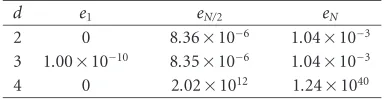
Table 6.3. Approximate error forExample 6.3.
d e1 eN/2 eN
2 0 8.36×10⁻⁶ 1.04×10⁻³
3 1.00×10⁻¹⁰ 8.35×10⁻⁶ 1.04×10⁻³
[image:16.468.145.320.350.400.2]4 0 2.02×10¹² 1.24×1040
Table 6.4. Approximate error forExample 6.1.
d e1 eN/2 eN
2 0 0 7.00×10⁻⁹
3 0 7.35×10⁻⁴ 6.23×10⁸
[image:16.468.139.328.438.489.2]4 0 8.02×10²³ 7.81×1065
Table 6.5. Approximate error forExample 6.2.
d e1 eN/2 eN
2 1.40×10⁻⁹ 3.32×10⁻⁴ 2.1×10⁻³
3 2.00×10⁻¹⁰ 4.52×10⁻² 3.87×10¹⁰
[image:16.468.140.329.525.575.2]4 8.00×10⁻¹⁰ 5.61×1027 5.48×1069
Table 6.6. Approximate error forExample 6.3.
d e1 eN/2 eN
2 0 8.36×10⁻⁶ 1.04×10⁻³
3 1.00×10⁻¹¹ 8.55×10⁻³ 7.34×10⁹
4 3.00×10⁻¹⁰ 2.34×1027 2.28×1069
From these numerical examples, we observe that a (3,d)-method is stable ford=2 and it is unstable ford=4. In the cased=3, this method is stable if the collocation parame-ters are uniformly distributed (i.e.,cj:=j/3, forj=1, 2, 3) as in case a, orc1=(3−
Table 6.7. Approximate error forExample 6.1.
d e1 eN/2 eN
2 1.55×10⁻⁶ 2.55×10⁻³ 2.46×10⁻²
3 9.30×10⁻⁶ 7.84×10²⁰ 1.80×1056
[image:17.468.139.329.178.229.2]4 1.01×10⁻⁴ 5.42×1052 5.03×10116
Table 6.8. Approximate error forExample 6.2.
d e1 eN/2 eN
2 1.6×10⁻⁹ 3.59×10⁻⁴ 1.00×10⁻⁴
3 1.10×10⁻⁹ 4.19×10¹⁷ 3.78×1053
[image:17.468.139.328.268.318.2]4 9.40×10⁻⁹ 4.80×1048 4.47×10112
Table 6.9. Approximate error forExample 6.3.
d e1 eN/2 eN
2 0 4.83×10⁻³ 3.65×10⁻²
3 0 3.40×10²³ 1.44×1059
4 2.00×10⁻⁴ 9.96×1052 9.40×10116
Table 6.10. Approximate error forExample 6.1.
d e1 eN/2 eN
2 1.00×10⁻⁹ 4.00×10⁻⁹ 1.20×10⁻⁸
3 0 0 7.00×10⁻⁹
4 0 4.45×10¹³ 5.12×1043
Table 6.11. Approximate error forExample 6.2.
d e1 eN/2 eN
2 1.10×10⁻⁹ 3.32×10⁻⁴ 2.11×10⁻³
3 6.00×10⁻¹⁰ 3.32×10⁻⁴ 2.11×10⁻³
4 3.00×10⁻¹⁰ 5.43×10¹⁶ 6.26×1046
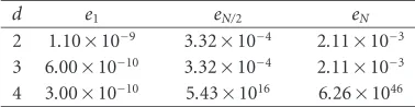
Table 6.12. Approximate error forExample 6.3.
d e1 eN/2 eN
2 0 8.36×10⁻⁶ 1.04×10⁻³
3 1.00×10⁻¹⁰ 8.36×10⁻⁶ 1.04×10⁻³
4 1.00×10⁻¹⁰ 3.06×10¹⁵ 3.54×1045
c2=(3 + √
[image:17.468.138.329.356.407.2] [image:17.468.139.328.447.496.2] [image:17.468.138.328.535.586.2]References
[1] H. Brunner,A survey of recent advances in the numerical treatment of Volterra integral and integro-differential equations, J. Comput. Appl. Math.8(1982), no. 3, 213–229.
[2] , Polynomial spline collocation methods for Volterra integrodifferential equations with weakly singular kernels, IMA J. Numer. Anal.6(1986), no. 2, 221–239.
[3] , The approximate solution of initial-value problems for general Volterra
integro-differential equations, Computing40(1988), no. 2, 125–137.
[4] H. Brunner and J. D. Lambert,Stability of numerical methods for Volterra integro-differential equations, Computing12(1974), no. 1, 75–89.
[5] H. Brunner, A. Pedas, and G. Vainikko,Piecewise polynomial collocation methods for linear Volterra integro-differential equations with weakly singular kernels, SIAM J. Numer. Anal.
39(2001), no. 3, 957–982.
[6] H. Brunner and P. J. van der Houwen,The Numerical Solution of Volterra Equations, CWI Monographs, vol. 3, North-Holland Publishing, Amsterdam, 1986.
[7] I. Danciu,Numerical stability of collocation methods for Volterra integro-differential equations, Rev. Anal. Num´er. Th´eor. Approx.26(1997), no. 1-2, 59–74.
[8] M. E. A. El-Tom,On the numerical stability of spline function approximations to solutions of Volterra integral equations of the second kind, Nordisk Tidskr. Informationsbehandling (BIT)14(1974), 136–143.
[9] A. Goldfine,Taylor series methods for the solution of Volterra integral and integro-differential equations, Math. Comp.31(1977), no. 139, 691–707.
[10] D. Harvey,Global approximations of initial value problems for speical second order ordinary dif-ferential equation, M. S. thesis, Dalhousie University, Halifax, Nova Scotia, 1971.
[11] M. Micul´a and G. Micula, Sur la r´esolution num´erique des ´equations int´egrales du type de Volterra de seconde esp`ece `a l’aide des fonctions splines, Studia Univ. Babes¸-Bolyai Ser. Math.-Mech.18(1973), no. 2, 65–68 (French).
[12] T. Lin, Y. Lin, M. Rao, and S. Zhang, Petrov-Galerkin methods for linear Volterra integro-differential equations, SIAM J. Numer. Anal.38(2000), no. 3, 937–963.
[13] V. Volterra,Theory of Functionals and of Integral and Integro-Differential Equations, Dover Pub-lications, New York, 1959.
Edris Rawashdeh: Department of Mathematics, Center for Applied Mathematics and Polymer Fluid Dynamics, Central Michigan University, Mount Pleasant, MI 48859, USA
E-mail address:[email protected]
Dave McDowell: Department of Mathematics, Center for Applied Mathematics and Polymer Fluid Dynamics, Central Michigan University, Mount Pleasant, MI 48859, USA
E-mail address:[email protected]
Leela Rakesh: Department of Mathematics, Center for Applied Mathematics and Polymer Fluid Dynamics, Central Michigan University, Mount Pleasant, MI 48859, USA