Using GIS Based Algorithms for GCMs’
Performance Evaluation
Salem S. Gharbia
Department of Civil, Structural and Environmental Engineering, Trinity College, Dublin
Dublin, Ireland [email protected]
Paul Johnston
Department of Civil, Structural and Environmental Engineering, Trinity College, Dublin
Dublin, Ireland [email protected]
Laurence Gill
Department of Civil, Structural and Environmental Engineering, Trinity College, Dublin
Dublin, Ireland [email protected]
Francesco Pilla
Department of Civil, Structural and Environmental Engineering, Trinity College, Dublin
Dublin, Ireland [email protected]
Abstract— General circulation models (GCMs) are used for estimating future climate scenarios, run on a very coarse scale, so the outputs from GCMs need to be downscaled to obtain a finer spatial resolution. This paper provides a methodology for GCM-Ensembles performance evaluation using a GIS platform by applying statistical spatial downscaling methods. Statistical downscaling methods were used in the projection process after validation and performance evaluation using several techniques such as Taylor diagram for each GCM-ensembles within independent sub-periods. Climate change projections for the Shannon River catchment in Ireland were developed for temperature and precipitation from multi-GCM ensembles for three future time intervals forcing by different Representative Concentration Pathways (RCP). The changes in temperature and precipitation were spatially projected at a very fine spatial scale.
Keywords—GCM; RCP; downscaling; climate change; GIS modelling
I. INTRODUCTION
Continued increases in greenhouse gas emissions at or above current rates would cause further warming during the 21st century which has been predicted to be greater than that observed during the 20th century [1, 2]. Projections of future climate change under scenarios obtained using climate system models have important practical significance, particularly for climate impact assessment studies and future emission control strategies [2, 3].
General circulation models (GCMs) are an essential technique in order to understand and predict the impacts of climate change. These numerical coupled models combine several earth systems including the atmosphere, oceans, land surface and sea-ice and offer considerable potential for the study of climate change and variability [4]. These climate models have been evolving steadily over the past several decades and in addition, are the most adapted tools for studying the impact of climate change at a regional scale. Recently, fully coupled
Atmosphere–Ocean GCMs, along with transient methods of forcing the concentration of greenhouse gases, have brought considerable improvement in the climate model results [5]. The current resolution of the GCMs, in average, is more than 2o, two polar degrees on the earth’s surface, for both directions in each pixel, which is close to a few hundred kilometers between grid points. Hence, GCMs typically provide output at grid boxes, which are tens of thousands of square kilometers in area, whereas the scale of interest with respect to most environmental system impact studies is of the order of a few hundred square kilometers, or even less. Several downscaling methodologies have thus been developed to deal with this problem of mismatch of spatial scales [5].
The spatial resolution mismatch between GCM outputs and the data requirements of environmental systems impacts models is a major problem. It is therefore necessary to produce some GCM-results processing to improve upon these global-scale models for impact studies. In order to overcome this obstacle, dynamical downscaling (regional climate models, RCMs) and statistical downscaling methods have been developed to fill this gap. RCMs are developed based on dynamic formulations using initial and time-dependent lateral boundary conditions of GCMs to achieve a higher spatial resolution at the expense of limited area modeling. The main problem of RCMs is the computational cost and so it is only available for limited regions. Moreover, despite improvements, outputs of RCMs are still too coarse for some practical applications, such as hydrological catchment impact studies, which need local and site-specific climate scenarios. Hence, statistical downscaling techniques have been developed to overcome these challenges [6-9]. In such environmental system impact studies, the emission scenario and the GCM are the main sources of uncertainty [10, 11]. Unfortunately, each step of the downscaling procedure also has associated uncertainties which all add up and constitute a cascade of uncertainty that must be
This research was funded by Trinity College, Dublin through Postgraduate Ussher Fellowship Award.
978-1-5090-0058-6/16/$31.00 ©2016 IEEE
Proceedings of the 18th Mediterranean Electrotechnical Conference MELECON 2016, Limassol, Cyprus, 18-20 April 2016
taken into account [8]. Recently, a set of scenarios known as Representative Concentration Pathways (RCPs) have been adopted by climate researchers to provide a range of possible futures for the evolution of atmospheric composition. These RCPs are competing and are going to replace earlier scenario-based projections of atmospheric composition. For example, the RCPs are being used to drive climate model simulations planned as part of the World Climate Research Programme’s Fifth Coupled Model Intercomparison Project (CMIP5) and other comparison exercises [12-15]. Since climate change projections obviously depend on the climate model results, the scientific community have set up an international project to compare these models. The various phases of the CMIP have grown steadily as testified both in terms of participants’ number and scientific impacts [16].
In this study, climate change projections for the Shannon River [17, 18] catchment are presented for several temperature and precipitation from multi-GCM ensembles for three future time intervals using a range of different Representative Concentration Pathways (RCPs). The projection process used a statistical downscaling procedure based on statistical relationships linking a set of large-scale atmospheric variables to regional climate variables in an observational calibration period. After validation and performance evaluation using several techniques such as the Taylor diagram for each GCM-ensemble within independent sub-periods, the established statistical relationships was used to predict the response of future regional climates from the simulated climate model changes of the large-scale variables. This paper presents the innovative use of a Geographical Information System (GIS) as a downscaling environment, which is unprecedented in literature.
II. METHODS
A multi-stage formulation modelling was carried out entirely within the Geographic Information System (GIS) environment in order to evaluate the performance of climate model multi-GCM ensembles and thereby adequately describe the future climate over Shannon river basin.
A set of weather variables (temperature and precipitation) were downscaled from climate change models at high quality resolution (cell size 50m*50m) from the GIS model and projected to three future time periods, the 2020s, 2050s and 2080s. Climate change models based on two different RCPs (using radiative forcing of 4.5 W/m2 and 8.5 W/m2 respectively) were produced from median and 3rd quartile of multi-GCM ensembles simulation results. The performance evaluation process for climate models results using the Taylor diagram and different statistical tests then lead to the development of high spatial resolution projected maps for temperature and precipitation.
A. Model Data
Observed daily data for precipitation and temperature were obtained from all available stations (96 stations) in the Shannon Catchment from the national Irish meteorology organisation (Met Éireann), for the period 1961-2014 (according to each station records). For baseline calculation purposes, data from
1961 to 2000 were used and the remaining data from 2000 to 2014 were used for the calibration and evaluation processes. Large-scale surface and atmospheric data were obtained from the datasets of the International Centre for Tropical Agriculture (CIAT) and the CGIAR Research Program on Climate Change, Agriculture and Food Security (CCAFS) [19-21]. Standardised reanalysis variables were then used as candidate predictor variables to calibrate the transfer functions, linking the large-scale surface and atmospheric variables to the observed stations data.
GCM data were obtained, for five models from the Hadley Centre, Canadian Centre for Climate Modelling and Analysis, Centre for Climate Research in Japan, the Commonwealth Scientific and Industrial Research Organization and National Centre for Atmospheric Research, USA for both representative concentration pathways RCP 4.5and RCP 8.5. All the modelled datasets exist on a common grid resolution that is varied between 125 Km and 370 Km and were obtained for the grid box representing Ireland in the GCM domain.
B. Selecting RCPs, modeling procesure and ensembles
Statistical or empirical downscaling is an alternative approach for obtaining regional-scale climate information from large-scale simulations to bridge the gap between global climate models and local impacts. The main idea behind statistical downscaling is to use statistical relationships to link resolved behaviors in GCMs with the climate in a study area. The study area’s size can be as small as a single point. This approach encompasses a range of statistical techniques as simple linear regression, delta change method, multiple regression, weather generators, canonical correlation analysis and artificial neural networks [22-28].
In this research, statistical tests (according to normality) for observed data, delta change and multiple regression methods were used to downscale future climate resulted from 50% (median) and 75% (3rd quartile) multi GCM-Ensembles forced by RCP 4.5 and RCP 8.5.
This paper presents a GIS-based python algorithm for GCM-Ensembles downscaling and performance evaluation simulations. This algorithm uses GIS as platform for simulation process through spatial geo-processors. The algorithm has a loop of process to downscale climate variable and evaluate the performance the designed GCM-Ensemble experiment. The observed weather data for Shannon, GCMs data and the selected RCPs are employed as a case study with different experiments in this GIS-based algorithm.
1. The algorithm spatial simulation steps are as follow: 2. Choose the GCMs that participated in the ensembles,
which is illustrated in the previous sections
3. Choose the forcing RCPs that targeted in each experiments.
4. Feed the multidimensional files for each global model experiment into the algorithm, which based on the GCMs simulation data.
order to fix the temporal resolution between all the experiments that participated in the ensemble.
6. Resample the grid size for each resulted gridded file from each experiment to unify the large scale resolutions.
7. Overlap the simulated grids for all GCMs that participated in the experiments.
8. Choose the downscaling method for each climatic variable in each experiment. In this case study, the developed GIS-based algorithm applies delta change method and multiple regression models as selected statistical downscaling methods under GIS platform. 9. Run a sub-algorithm for the selected downscaling
method for the specific experiment with the observed data as input.
10. Evaluate the results for each experiment through statistics and Tylor diagram.
Ensembles or weighting of the downscaled results was developed to overcome different GCM results risk in climate change projections. This ensembles or weighting was based on the individual GCMs ability to reproduce the properties of the observed climate. The modified impacts relevant climate prediction index is weighted based on the individual GCMs ability to reproduce the properties of the observed climate and is derived from the root-mean-square difference between modelled and observed climatological data [29, 30], median and 75 percentile (3rd quartile), assessed over the baseline period. The median and 75 percentile ensembles, produced from the weighted median and 75 percentile results for multi-GCM described above, were developed for Shannon catchment and assessed over the baseline.
The delta method or change factor is the ratio between GCM simulations of future and current climate. It is used as a multiplicative factor to obtain future regional conditions so that the differences between the control and future GCM simulations are applied to baseline observations by adding or scaling the mean climatic to each time step. The method assumes that GCMs more accurately simulate relative change more than absolute values. In addition, the change factors only scale the mean, maximum and minimum of the climatic variables, ignoring changes in variability and assuming the spatial pattern of climate will remain constant [4].
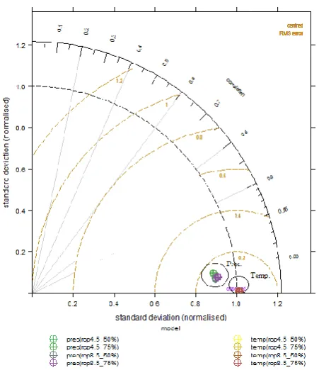
In order to evaluate the performance of models in a single diagram, Taylor diagrams [31] provide an efficient way of graphically summarizing how closely a model or ensemble fits observations. The similarity between two patterns is quantified in terms of their correlation, their centered root-mean-square difference and the amplitude of their variations. In this paper Taylor diagrams have been used to validate and evaluate the performance of climate models and ensembles.
III. RESULTS AND DISCUTIONS
In order to validate the climate models results, observed data for each modeled climate variable for the 1961-2014 periods were used for the validation process. High correlations were obtained for climate models validation as shown in Table (1)
[image:3.595.302.564.103.168.2]which illustrated statistical tests results (R2 values) for all modeled variable for Shannon catchment.
Table 1: climate models validation statistical tests results.
Predictands Predictors R R2 Adjusted
R2
Standard error of
the estimate
Temperature Temperature 0.997 0.995 0.994 0.02047
Precipitation Precipitation 0.997 0.994 0.993 1.58028
For climate models and ensembles performance evaluations, Taylor diagrams and box-whisker plots have been prepared for each modeled monthly climate variable. In the Taylor diagram (Fig. 1), statistics for 8 models were computed with a colored point assigned to each model. The position of each point appearing on the plot quantifies how closely the model's simulated results match the observations. First of all, it can be seen that the pattern correlations are generally high (higher than 0.7 in all cases). Secondly, one can notice that the variance is generally underestimated by the models, whatever the climatic variable, RCP or ensemble. This was actually expected from the high values of R-square for validation period. It is also interesting to note that there is high coherence between the models: they share similar qualities or deficiencies (see the clusters of color points for each climatic variable). In Taylor diagram the horizontal and vertical axes represent the ratio of the standard deviations of the reference and simulated fields. The radial axis indicates the spatial correlation between the reference and simulated fields. The distance between the origin and any point is proportional to the RMSE
.
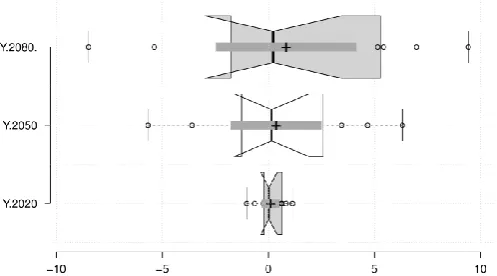
[image:3.595.321.547.417.678.2]Also for the multi-GCM ensembles performance evaluation, Figures (2-9) were developed for each projected climatic variables and for each climate scenario changes from baseline values. Each table has box-whisker diagrams in which the center lines show the medians, the box limits indicate the 25th and 75th percentiles as determined by R software, the whiskers extend to 1.5 times the interquartile range from the 25th and 75th percentiles, outliers are represented by dots, crosses represent sample means, bars indicate 95% confidence intervals of the means, and notches are defined as +/-1.58* inter quartile range /sqrt(n) and represent the 95% confidence interval for each median. Non-overlapping notches give 95% confidence that two medians are different. It is clear that the absolute values and the changes from baseline values for each climate variable increase with increasing projected years and by moving from left to right side in each table from RCP 4.5 (50%) to RCP 8.5 (75%).
Figure 2: Monthly differences from baseline values box-whisker plots for each year of predicted temperature (oC) forced by RCP 4.5(50%).
Figure 3: Monthly differences from baseline values box-whisker plots for each year of predicted temperature (oC) forced by RCP 4.5(75%).
Figure 4: Monthly differences from baseline values box-whisker plots for each year of predicted temperature (oC) forced by RCP 8.5(50%).
Figure 5: Monthly differences from baseline values box-whisker plots for each year of predicted temperature (oC) forced by RCP 8.5(75%).
[image:4.595.307.549.240.368.2] [image:4.595.37.287.269.397.2] [image:4.595.308.557.431.569.2] [image:4.595.39.286.461.595.2]Figure 7: Monthly differences from baseline values box-whisker plots for each year of predicted precipitation (mm) forced by RCP 4.5(75%).
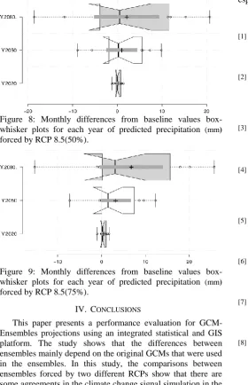
Figure 8: Monthly differences from baseline values box-whisker plots for each year of predicted precipitation (mm) forced by RCP 8.5(50%).
Figure 9: Monthly differences from baseline values box-whisker plots for each year of predicted precipitation (mm) forced by RCP 8.5(75%).
IV. CONCLUSIONS
This paper presents a performance evaluation for GCM-Ensembles projections using an integrated statistical and GIS platform. The study shows that the differences between ensembles mainly depend on the original GCMs that were used in the ensembles. In this study, the comparisons between ensembles forced by two different RCPs show that there are some agreements in the climate change signal simulation in the study area. However, it is not easy to locate the changes with spatially precision and accuracy especially for precipitation,
which makes the use of such results for decision-making difficult by relevant stakeholders and practitioners.
The study of temperature shows that there are important differences between the ensembles, especially in summer months. These differences may of interest because of how they affect the accuracy of the simulations of hydrological processes. The study shows that downscaling is a crucial step when only one climate model is used to study the impacts of climate change because of the wide uncertainty related to GCM choosing process; it is important to apply multi-climate model in climate change simulation studies especially on hydrological impacts studies.
The paper outlines the importance of using a GIS platform with raster data as a downscaling environment in order to derive very fine scale resolution future-projected changes in climate, especially for hydrological modeling purposes.
REFERENCES
[1] Solomon, S., Climate change 2007-the physical science basis: Working group I contribution to the
fourth assessment report of the IPCC. Vol. 4. 2007:
Cambridge University Press.
[2] Stocker, T.F., et al., Climate change 2013: The
physical science basis. Intergovernmental Panel on
Climate Change, Working Group I Contribution to the IPCC Fifth Assessment Report (AR5)(Cambridge Univ Press, New York), 2013.
[3] Xiaoge, X., et al., Climate change projections over East Asia with BCC_CSM1. 1 climate model under
RCP scenarios. 気象集誌. 第 2 輯, 2013. 91(4): p.
413-429.
[4] Fowler, H., S. Blenkinsop, and C. Tebaldi, Linking climate change modelling to impacts studies: recent advances in downscaling techniques for hydrological
modelling. International Journal of Climatology,
2007. 27(12): p. 1547-1578.
[5] Tripathi, S., V. Srinivas, and R.S. Nanjundiah, Downscaling of precipitation for climate change scenarios: a support vector machine approach. Journal of hydrology, 2006. 330(3): p. 621-640. [6] Chen, J., F.P. Brissette, and R. Leconte, Uncertainty
of downscaling method in quantifying the impact of
climate change on hydrology. Journal of hydrology,
2011. 401(3–4): p. 190-202.
[7] Minville, M., F. Brissette, and R. Leconte, Uncertainty of the impact of climate change on the
hydrology of a nordic watershed. Journal of
hydrology, 2008. 358(1–2): p. 70-83.
[8] Quintana Seguí, P., et al., Comparison of three downscaling methods in simulating the impact of climate change on the hydrology of Mediterranean
basins. Journal of hydrology, 2010. 383(1–2): p.
111-124.
[image:5.595.39.287.57.189.2] [image:5.595.37.318.245.680.2]investigations of climate change. Journal of hydrology, 2011. 402(3–4): p. 193-205.
[10] Maurer, E. and H. Hidalgo, Utility of daily vs.
monthly large-scale climate data: an
intercomparison of two statistical downscaling
methods. Hydrology and Earth System Sciences,
2008. 12(2): p. 551-563.
[11] Boé, J., et al., Statistical and dynamical downscaling
of the Seine basin climate for hydro‐meteorological
studies. International Journal of Climatology, 2007.
27(12): p. 1643-1655.
[12] Meinshausen, M., et al., The RCP greenhouse gas concentrations and their extensions from 1765 to
2300. Climatic change, 2011. 109(1-2): p. 213-241.
[13] Moss, R.H., et al., Towards new scenarios for analysis of emissions, climate change, impacts, and
response strategies. 2008.
[14] Moss, R.H., et al., The next generation of scenarios
for climate change research and assessment. Nature,
2010. 463(7282): p. 747-756.
[15] Taylor, K.E., R.J. Stouffer, and G.A. Meehl, A
summary of the CMIP5 experiment design. WCRP,
submitted, 2009.
[16] Dufresne, J.-L., et al., Climate change projections using the IPSL-CM5 Earth System Model: from
CMIP3 to CMIP5. Climate Dynamics, 2013.
40(9-10): p. 2123-2165.
[17] McCarthy, T., et al., Long-term effects of hydropower installations and associated river regulation on River
Shannon eel populations: mitigation and
management. Hydrobiologia, 2008. 609(1): p.
109-124.
[18] OPW, Shannon Catchment-based Flood Risk
Assesment and Managment (CFRAM) Study 2011,
The Office of Public Work (OPW): , Dublin, Ireland. [19] Mitchell, T. and T. Osborn, ClimGen: a flexible tool
for generating monthly climate data sets and
scenarios. Tyndall Centre for Climate Change
Research Working Paper, 2005.
[20] Ramirez, J. and A. Jarvis, High resolution statistically downscaled future climate surfaces. International Center for Tropical Agriculture (CIAT), 2008.
[21] Wilby, R.L. and T. Wigley, Downscaling general circulation model output: a review of methods and
limitations. Progress in Physical Geography, 1997.
21(4): p. 530-548.
[22] Salathe, E.P., P.W. Mote, and M.W. Wiley, Review of scenario selection and downscaling methods for the assessment of climate change impacts on hydrology in the United States Pacific Northwest.
International Journal of Climatology, 2007. 27(12): p. 1611-1621.
[23] Kattenberg, A., et al., Climate models—projections of
future climate. Climate Change 1995: The Science of
Climate Change. Contribution of Working Group I to the Second Assessment Report of the Intergovernmental Panel on Climate Change, 1996: p. 285-357.
[24] Hewitson, B. and R. Crane, Consensus between GCM
climate change projections with empirical
downscaling: precipitation downscaling over South
Africa. International Journal of Climatology, 2006.
26(10): p. 1315-1337.
[25] Joubert, A. and B. Hewitson, Simulating present and future climates of southern Africa using general
circulation models. Progress in Physical Geography,
1997. 21(1): p. 51-78.
[26] Giorgi, F., et al., Regional climate
information-evaluation and projections. Climate Change 2001:
The Scientific Basis. Contribution of Working Group to the Third Assessment Report of the Intergouvernmental Panel on Climate Change [Houghton, JT et al.(eds)]. Cambridge University Press, Cambridge, United Kongdom and New York, US, 2001.
[27] von Storch, H., E. Zorita, and U. Cubasch, Downscaling of global climate change estimates to regional scales: an application to Iberian rainfall in
wintertime. Journal of Climate, 1993. 6(6): p.
1161-1171.
[28] Crane, R.G. and B.C. Hewitson, Doubled CO2 precipitation changes for the Susquehanna Basin:
Down‐scaling from the Genesis general circulation
model. International Journal of Climatology, 1998.
18(1): p. 65-76.
[29] Hulme, M. and T.R. Carter. Representing uncertainty
in climate change scenarios and impact studies. in
Representing uncertainty in climate change scenarios and impact studies (Proc. ECLAT-2 Helsinki Workshop, 14-16 April, 1999 (Eds. T. Carter, M. Hulme and D. Viner). 128pp Climatic Research Unit,
Norwich, UK. 1999.
[30] Wilby, R.L. and I. Harris, A framework for assessing
uncertainties in climate change impacts: Low‐flow
scenarios for the River Thames, UK. Water
Resources Research, 2006. 42(2).
[31] Taylor, K.E., Summarizing multiple aspects of model
performance in a single diagram. Journal of