BIROn - Birkbeck Institutional Research Online
Smith, Ron P. and Pesaran, M.H. (2019) The role of factor strength and
pricing errors for estimation and inference in asset pricing models. Working
Paper. Munich Society for the Promotion of Economic Research - CESifo
GmbH, Munich, Germany.
Downloaded from:
Usage Guidelines:
Please refer to usage guidelines at or alternatively
7919
2019
October 2019
The Role of Factor Strength
and Pricing Errors for
Estima-tion and Inference in Asset
Pricing Models
Impressum:
CESifo Working Papers
ISSN 2364-1428 (electronic version)
Publisher and distributor: Munich Society for the Promotion of Economic Research - CESifo GmbH
The international platform of Ludwigs-Maximilians University’s Center for Economic Studies and the ifo Institute
Poschingerstr. 5, 81679 Munich, Germany
Telephone +49 (0)89 2180-2740, Telefax +49 (0)89 2180-17845, email [email protected] Editor: Clemens Fuest
www.cesifo-group.org/wp
An electronic version of the paper may be downloaded · from the SSRN website: www.SSRN.com
· from the RePEc website: www.RePEc.org
CESifo Working Paper No. 7919 Category 12: Empirical and Theoretical Methods
The Role of Factor Strength and Pricing Errors for
Estimation and Inference in Asset Pricing Models
Abstract
In this paper we are concerned with the role of factor strength and pricing errors in asset pricing models, and their implications for identification and estimation of risk premia. We establish an explicit relationship between the pricing errors and the presence of weak factors that are correlated with stochastic discount factor. We introduce a measure of factor strength, and distinguish between observed factors and unobserved factors. We show that unobserved factors matter for pricing if they are correlated with the discount factor, and relate the strength of the weak factors to the strength (pervasiveness) of non-zero pricing errors. We then show, that even when the factor loadings are known, the risk premia of a factor can be consistently estimated only if it is strong and if the pricing errors are weak. Similar results hold when factor loadings are estimated, irrespective of whether individual returns or portfolio returns are used. We derive distributional results for two pass estimators of risk premia, allowing for non-zero pricing errors. We show that for inference on risk premia the pricing errors must be sufficiently weak. We consider both when n (the number of securities) is large and T (the number of time periods) is short, and the case of large n and T. Large n is required for consistent estimation of risk premia, whereas the choice of short T is intended to reduce the possibility of time variations in the factor loadings. We provide monthly rolling estimates of the factor strengths for the three Fama-French factors over the period 1989-2018.
JEL-Codes: C380, G120.
Keywords: arbitrage pricing theory, APT, factor strength, identification of risk premia, two-pass regressions, Fama-French factors.
M. Hashem Pesaran University of Southern California
Los Angeles / CA / USA [email protected]
Ron P. Smith
Birkbeck, University of London London / United Kingdom
October 16, 2019
1
Introduction
Asset pricing models tend to attribute di¤erences in expected returns to di¤erences in exposure to systematic risk factors. For instance, the arbitrage pricing theory (APT) formalised by Ross (1976), assumes that there are many assets, with returns determined by a small number of factors, and that competitive markets do not permit arbitrage opportunities. Thus returns can be split into two components: non-diversi…able systematic risk from exposure to the common factors, and idiosyncratic risk, which can be eliminated in a well diversi…ed portfolio. Assets with similar risk factors are close substitutes so should have similar returns. In this linear return generating process, expected excess returns are proportional to systematic risk, measured by factor loadings and risk premia are the coe¢ cients of such loadings. Chamberlain and Rothschild (1983) extend the theory to an approximate factor structure and provide a rigorous treatment of the case of in…nitely many assets. Wei (1988) links the APT to the capital asset pricing model, CAPM. Within the context of such models, the risk factors and their loadings have to be identi…ed and the risk premia associated with them estimated. The standard procedure is to estimate factor loadings from a …rst-pass time series regression of excess returns for each asset, and in a second-pass the Fama-MacBeth (1973) type cross section regression is used to price the factors and obtain the risk premia.
In this paper we are concerned with the role of factor strength and pricing errors in asset pricing models, and their implications for identi…cation and estimation of risk premia. We distinguish between strong and weak factors that underlie the APT by relating them to the stochastic discount factor, mt, used to price securities within the inter-temporal asset pricing
models. We introduce a measure of factor strength denoted by , and distinguish between observed factors, ft = (f1t; f2t; :::; fkt)0, with strengths f = ( f1; f2; :::; fk)
0, and unobserved
factors (included in the idiosyncratic errors) labelled gt = (g1t; g2t; :::; gkgt)0 with strengths
g = g1; g2; :::; gkg
0
. Non-zero pricing errors arise when the errors in the factor model are correlated with mt. By decomposing the errors into a part which is correlated with mt, and a
purely idiosyncratic part, "t; which is not, we show that the APT equilibrium condition only
bounds the cross correlation of the …rst part and does not impose any restrictions on the cross correlation of the purely idiosyncratic part. Such cross correlations could arise at times of …nancial crises possibly due to herding and other forms of correlated behavior that stem from non-fundamental considerations.
We de…ne the strength of a given factor, say ft, by the exponent f in the following norm
condition
n
X
i=1
i n
2
= n f ; (1)
where i is the loading of ft on the ith security, n = n 1
Pn
i=1 i, and n f denotes the
expansion rate of the dispersion measure Pni=1 i n 2
in terms of n. To motivate the use of in the analysis of factor pricing we …rst generalise Ross’s APT equilibrium condition. Ross required pricing errors, denoted by i for security i, to be bounded, in the sense that
Pn
i=1 2
i <1. We show that this condition can be relaxed to n
X
i=1 2
i =O(n ); (2)
above relates to unobserved common factors that are correlated with the discount factor). The exponent of the pricing errors, , is to be contrasted with the exponent of factor strength . For a factor to be strong it is necessary that its e¤ect is pervasive on all securities. In terms of (1), this requires f = 1. Whilst, the pricing errors must not be pervasive, requiring that <1.
Note that the standard order condition, O( ), used in (2) allows zero pricing errors ( i = 0 for
all i), and ( ) ensures that the e¤ects of ft are su¢ ciently pervasive when f = 1.
Having linked the APT to the inter-temporal asset pricing condition, and given the distinc-tion between ft and gt factors, we then consider the problem of identi…cation of risk premia,
initially assuming known factor loadings, using an approximate linear factor model. We show that for large n the risk premia can be pn consistently estimated if the factors all have maxi-mum strength with f = 1, and the pricing errors are weak such that < 1. In the literature
the distinction between risk factors and pricing errors is not always as clear-cut. For instance Stambaugh & Yuan (2017, p. 1273) say "there need not be a clear distinction between mispric-ing and risk compensation as alternative motivations for factor models of expected returns." They use the example of "noise-trader" sentiment, but if such sentiment is su¢ ciently pervasive it constitutes a factor that may be priced.
We further establish that these conditions for the identi…cation of the risk premia are un-a¤ected if one uses portfolios as compared to individual securities, as is often done in the empirical literature. There is a belief that the …rst stage estimation of the betas causes an errors in variables problem in the second stage and that the construction of portfolios mitigates this problem. We regard this as a generated regressor problem, which is rather di¤erent, and like Ang et al. (2019) argue that forming portfolios wastes information. Nonetheless we analyse both cases: using individual assets and using portfolios.
We then move to the more interesting case where the factor loadings are unknown, and derive conditions under which the risk premia can be identi…ed. Using the two pass estimator of Fama-MacBeth, we show that risk premia are only identi…ed if both n and T ! 1, such that n=T ! , with0< <1, all factors have maximum strength, and the pricing errors are su¢ ciently weak. The large T results on estimation of risk premia obtained in the literature, and reviewed for example by Jagannathan, Skoulakis & Wang (2010), only apply if it is assumed that pricing errors are all zero (namely i = 0 for all i). In the presence of non-zero pricing
errors, we need n ! 1, and it is not su¢ cient to consider large T asymptotics. When T is …xed and n ! 1, we consider a bias-corrected version of the two pass estimator and show that in this case risk premia are not identi…ed and one can only consistently estimate what Shanken (1992, p. 6) has termed "ex-post prices of risk". For this result, we still require all factors to have maximum strength and the pricing errors to be su¢ ciently weak. Finally, we consider the limiting distributions of the bias corrected estimator, centred around the ex post risk premia, for a …xed T and as n ! 1, as well as when n; T ! 1. Under the former we show that the limiting distribution of bias-corrected two pass estimator exists, but need not be Gaussian due to the error cross sectional dependence. In contrast, under joint n and
T asymptotics, the estimator is asymptotically normal, and does not depend on the errors of individual securities, but is primarily driven by the time series properties of the factors. In both cases, to ensure that the asymptotic distributions do not depend on the pricing errors, we must have Pni=1j ij = O(n ), with < 1=2, which is much more restrictive than the condition
needed on for consistent estimation of risk premia.
2016 and BKP 2019a) on measures of cross-sectional dependence in large panels. Whereas BKP (2019b) are concerned with estimation and inference about the strength of a factor, as noted above this paper is concerned with a di¤erent issue, the theoretical role of factor strength and pricing errors in asset pricing models and estimation and inference about risk premia in such models.
BKP (2019b) show that the strength of a factor can be estimated from the proportion of statistically signi…cant loadings across a large number of securities. Let n be the number of securities and Dn the number of signi…cant loadings, then n = Dn=n is the proportion
of non-zero loadings and the measure of factor strength is the logarithmic transform: f =
1 + ln( n)=ln(n). The critical values of the tests are suitably adjusted to allow for multiple
testing and it is shown that this estimator is consistent. Using Monte Carlo experiments, BKP also show that the estimates of the factor strengths are quite accurate when the factors are su¢ ciently strong, even for moderate sample sizes. It is important to note that for identi…cation of risk premia, the crucial measure is f not n: Since n=n 1; then if does not equal one,
the proportion of the n securities that have non-zero loadings goes to zero withn, albeit rather slowly at log rate. For the proportion of non-zero loadings to be constant as n rises, it is required that = 1.
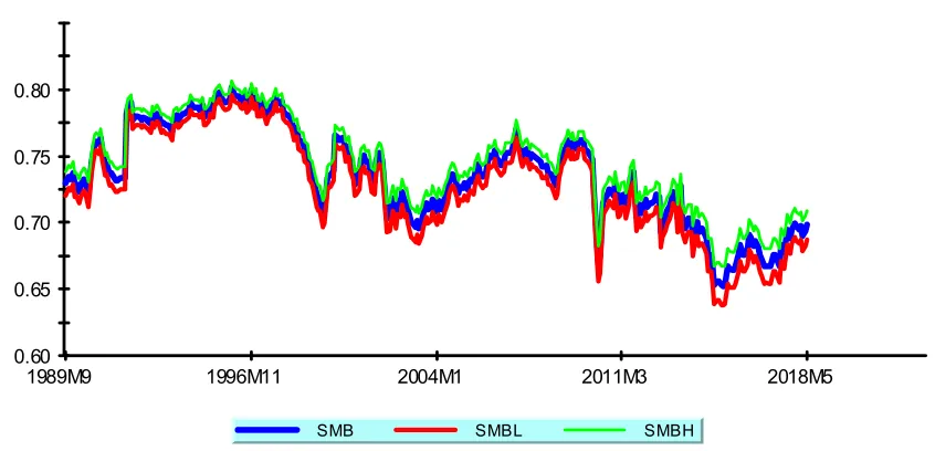
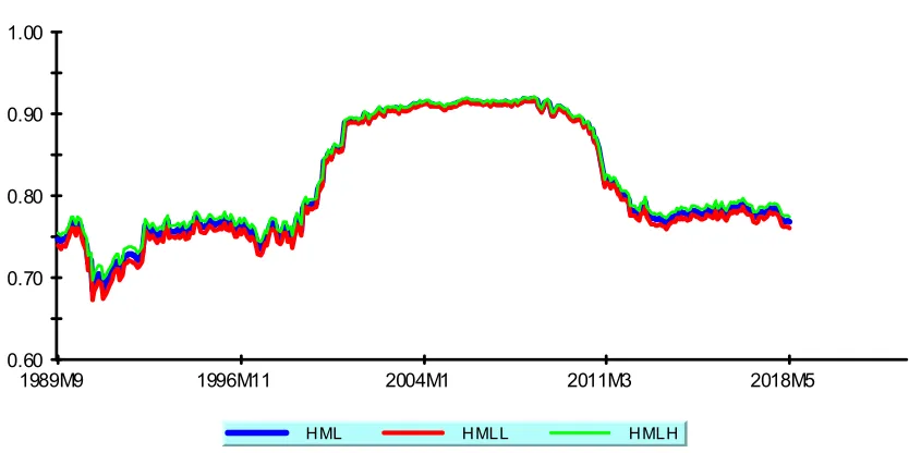
We conclude the paper with an empirical application, using the estimator of proposed by BKP (2019b). For each monthly time point ending from September 1989 to May 2018, the stocks in the S&P 500 at that month with a 10 year history are identi…ed. Then a time series regression is estimated regressing the excess return for each stock on a constant and the three Fama & French (1993) factors. These are the market factor, the size factor, small minus big (SMB), and the value factor, high book to market minus low (HML). The estimated strength of the market factor is either one or very close to one. The market factor is always much stronger than the other two factors, whose strength varies substantially over the period considered, and tend to vary between 0:65and 0:9. The con…dence bounds around the estimates of the factor strengths are tight and the outcomes are reasonably robust to the choice of estimation window. Throughout this paper we assume that the potential factors are known. There is no shortage of suggested factors, Harvey and Liu (2019) document a "factor zoo" of over 400 suggested factors in early 2019. They may be observable macro factors like those suggested by Chen, Roll & Ross (1986); obtained from factor analysis of the returns as discussed in Lehmann & Modest (2005); based on asset pricing anomalies like the Fama-French factors; or obtained in some other way. Fama & French (2018) discuss some issues in choosing factors. We are concerned with establishing the theoretical role of factor strengths and providing estimates of them, not with the issue of how to select factors.
Our analysis has important practical implications for estimating factor risk premia from second-pass cross section regressions of average returns on factor loadings. The factors used in the …rst-pass time series regressions to estimate the loadings must be su¢ ciently strong. The
strength of the factor ought to be measured using rolling windows estimates of the parameter ;
as illustrated in Section 5. Only factors with an average strength of 2=3; should be included
in the analysis. Estimates of the risk premia for factors with = 2=3 will be consistent at
the rate of n1=3, and thus will be di¢ cult to price unless n is very large indeed. The situation
is clearly worse for < 2=3; when estimates of also become less reliable due to increased
The rest of the paper is organized as follows. Section 2 sets out the factor model and derives the APT pricing errors by imposing the equilibrium conditions from standard pricing theory. Section 3 discusses the identi…cation of the risk premia for the factors from a cross section when the factor loadings are known. It considers both the cases where the observations are individual securities and where they are portfolios. Section 4 discusses the case where the factor loadings are unknown and have to be estimated in the …rst-pass time series regressions. Again it considers individual securities and portfolios. Section 5 presents the estimates of time-varying factor strength. Section 6 has some concluding comments. Lemmas, proofs and related results are provided in appendices.
Notation: Generic positive …nite constants are denoted byCwhen large, andcwhen small. They can take di¤erent values at di¤erent instances. !p denotes convergence in probability as
n; T ! 1. max(A) and min(A) denote the maximum and minimum eigenvalues of matrix A. A > 0 denotes that A is a positive de…nite matrix. kAk = max1=2 (A0A) and kAkF =
[T r(A0A)]1=2 denote the spectral and Frobenius norm of matrix A, respectively. If ffng1n=1
is any real sequence and fgng1n=1 is a sequences of positive real numbers, then fn = O(gn),
if there exists C such that jfnj=gn C for all n. fn = o(gn) if fn=gn ! 0 as n ! 1.
Similarly, fn =Op(gn)if fn=gnis stochastically bounded, andfn=op(gn);if fn=gn!p 0, where
!pdenotes convergence in probability. If ffng1n=1 and fgng1n=1 are both positive sequences of
real numbers, then fn = (gn) if there exists n0 1 and positive …nite constants C0 and C1,
such that infn n0(fn=gn) C0;and supn n0(fn=gn) C1.
2
APT, equilibrium pricing theory and non-zero pricing
errors
Non-zero pricing errors have a central role in this paper. This section sets out the factor model and derives the APT pricing errors in terms of the correlation of the discount factor with the idiosyncratic component of excess returns. We achieve this by imposing the equilibrium conditions from standard pricing theory on the linear multi-factor model used by Ross and others in the literature. We show that non-zero pricing errors arise when there are factors in the idiosyncratic (error) part of excess returns that are correlated with the stochastic discount factor.
To establish our main result we follow the literature and assume that returns, ri;t+1; i =
1;2; :::n, are generated according to the following linear multi-factor model1
ri;t+1 r f
t =ait+ k
X
j=1
it;jfj;t+1+ui;t+1; for i= 1;2; :::; n; (3)
where rtf is the risk free rate; ait are the intercepts in the factor model; fj;t+1; j = 1;2; :::; k
are the common factors with associated factor loadings, it;j; and ui;t+1 is the idiosyncratic
component of asset return. The model can be written more compactly as
ri;t+1 rft =ait+
0
itft+1+ui;t+1; (4)
1Because the number of assets may change through time, we could have a time varying n
where it = ( it;1; it;2; :::; it;k)0, and ft+1 = (f1;t+1; f2;t+1; :::; fk;t+1)0. We assume the errors of
the factor model, ui;t+1, are martingale di¤erences, Et(ui;t+1) = 0, and have …nite conditional
variances, and are cross-sectionally weakly correlated. We explore the relationship between
ui;t+1 and the pricing errors in detail below. But at this stage we view ui;t+1 as errors in the
statistical factor model used to represent the time series variations of individual excess returns. The cross-sectional dependence of the individual returns is captured by the common factors, ft+1, and the degree of cross-sectional dependence of the errors, ui;t+1. Denoting the n 1
vector of errors by un;t+1 = (u1;t+1; u2;t+1; :::; un;t+1)0, and its covariance matrix by u;nt =
Et un;t+1u0n;t+1 , an overall measure of cross dependence of the errors is given by the rate at
which max( u;nt) rises with n. We denote this rate by t; , and relate it to the pervasiveness
of the pricing errors under APT. Ross (1976) assumedui;t+1 were cross sectionally independent,
Chamberlain & Rothschild (1983) weakened this to an approximate factor model that requires
max( u;nt)< C in n and t, which corresponds to setting t; = 0 for all t.
In what follows we require that t; <1, and assume that the factors,ft+1; are strong in the
sense that t;fj de…ned by
2
n
X
i=1
it;j tj 2
= n t;fj , for j = 1;2; :::; k; (5)
are equal to unity. The main result of the APT can now be written as the cross section return regression
Et ri;t+1 rtf =
0
it t+ it; (6)
where t is thek 1 vector of factor risk prices (or risk premia), and it is the pricing error of
the ith security, assumed to satisfy the APT condition (18) of Ross (1976), namely
supt n
X
i=1 2
it < C: (7)
To relate the pricing errors to the idiosyncratic component of returns we use standard results from intertemporal asset pricing theory that require equilibrium prices, Pit, to be set as the
expected discounted value of the payo¤, Pi;t+1+Di;t+1. Denoting the holding period return by
ri;t+1 = ( Pi;t+1+Di;t+1)=Pit, the basic equilibrium pricing equation can be written as
Et
h
mt+1(ri;t+1 rft)
i
= 0; (8)
where mt+1 is the stochastic discount factor used to price all assets in the market, andrft is the
risk free rate.3 We also note that
Et(mt+1) = 1=(1 +rtf)>0: (9)
To derive conditions under which the factor model (4) also satis…es the equilibrium condi-tions, substituting for ri;t+1 rft from (4) in (8), we have
aitEt(mt+1) +
0
itEt(mt+1ft+1) +Et(mt+1ui;t+1) = 0:
2See also (1) and the related discussion in the Introduction. 3Under consumption based asset pricing m
Now noting that Et(mt+1)>0; (see (9)), then ait can be solved as
ait =
1 Et(mt+1)
h 0
itEt(mt+1ft+1) +Et(mt+1ui;t+1)
i
: (10)
Imposing this restriction by substituting the above expression for ait back in (3) yields
ri;t+1 rft =
0
it ft+1
Et(mt+1ft+1)
Et(mt+1)
Et(mt+1ui;t+1)
Et(mt+1)
+ui;t+1: (11)
Taking conditional expectations of both sides of the above and noting that Et(ui;t+1) = 0, we
now have
Et ri;t+1 rft =
0
itEt ft+1
Et(mt+1ft+1)
Et(mt+1)
Et(mt+1ui;t+1)
Et(mt+1)
:
Matching this result with the APT equilibrium condition given by (6), we obtain the following expressions for the risk premia and the pricing errors
t =Et ft+1
Et(mt+1ft+1)
Et(mt+1)
= Covt(mt+1;ft+1) Et(mt+1)
; (12)
and
it=
Et(mt+1ui;t+1)
Et(mt+1)
, fori= 1;2; :::; n: (13)
The pricing errors are zero only if ui;t+1 and mt+1 are conditionally uncorrelated. Also their
identi…cation requires knowledge of the stochastic discount factor as well as the factors. But (13) does not place any restrictions on the relationships between the pricing errors and the factor loadings, which as we shall see is an important consideration for estimation of risk premia.
For a better insight into the factors that could lead to non-zero pricing errors, it is useful to decomposeui;t+1into three mean zero components: (i) a set ofkg unobserved factors denoted by gt+1 = (g1;t+1; g2;t+1; :::; gkg;t+1)0 withEt(gt+1) =0, that are correlated with the discount factor,
mt+1; (ii) a set ofkhunobserved factorsht+1 = (h1;t+1; h2;t+1; :::; hkh;t+1)
0 withE
t(ht+1) = 0that
areuncorrelated withmt+1 ; and (iii) idiosyncratic errors,"i;t+1, that are also uncorrelated with
mt+1;but could be cross-sectionally correlated without having a common factor representation.
Such dependencies could arise from local or network spillover e¤ects that are unrelated to
mt+1. The error components that do not depend on mt+1, namely ht+1 and "i;t+1, can still
become highly correlated across securities at times of …nancial crises, for example, possibly due to herding behavior or correlated beliefs that cause asset returns to move together in a way that is unrelated to the economy’s fundamentals. The unobserved factors gt+1 and ht+1 are
distinguished from the observed risk factors, ft, in two respects. First, since gt+1 and ht+1 are
martingale di¤erence processes thus having zero means, whilst risk factors, ft+1, need not have
zero means; and most importantly the two sets of factors could di¤er in their strengths. As we shall see, the APT theory requires the unobserved factors that are correlated with mt+1
must be weak and the risk factors must be strong. It does not impose any restrictions on the degree of cross-sectional dependence of the returns that are due to ht+1 and/or "i;t+1, the two
components of ui;t+1 that are unrelated to mt+1.
More speci…cally let
ui;t+1 = kg
X
j=1
it;jgj;t+1+ kh
X
j=1
where it= ( it;1; it;2; :::; it;kg)0 and it= ( it;1; it;2; :::; it;kh)
0 arek
g 1 and h 1vectors
of loadings associated to gt+1 and ht+1, respectively. Now using (14) in (13) and noting that
ht+1 and "i;t+1 are uncorrelated withmt+1, we have
it= kg
X
j=1
j;t+1 it;j =
0
t+1 it; (15)
where t+1 =Covt(gt+1; mt+1)=Et(mt+1)6=0. Therefore, the pricing errors arise solely due to
the non-zero correlation of gt+1 and mt+1:4 Using (15) in (13) we have
n
X
i=1 2
it= 0t+1 n
X
i=1 it 0it
!
t+1: (16)
It is clear that the leading terms of above expression are given by Pni=1 2
it;j = O(n t;gj); for
j = 1;2; :::; kg, where t;gj is the strength of factor gj;t+1: The strength of the pricing errors,
given by Pni=1 2
it = O(n t); is determined by the strongest of the weak factors, gj;t with t = supj( t;gj): Below we will see that to identify the risk premia, the factors fjt must be
strong with t;fj = 1, for all j = 1;2; ::; k, and for estimation and inference on the risk premia
the pricing errors must be su¢ ciently weak, t= supj( t;gj)<1=2.
The above derivations link the pervasiveness of the pricing errors to the presence of weak factors in the idiosyncratic errors, ui;t+1, of the return equations. The equilibrium pricing
condition of Ross (1976), given by (7), is satis…ed if the factorsgt+1 that enter the idiosyncratic
component of the returns have zero strength, in the sense that t;gj = 0;for all j. Our analysis
relaxes this condition by requiring that t;gj < 1=2. Also the components of ui;t+1 in (14),
ht+1 and "i;t+1;which do not depend onmt+1;can be more strongly cross-correlated, because of
herding or correlated beliefs, than the …rst component,gt+1which depends on the fundamentals,
and is governed by the APT condition, (7).
3
Identi…cation of risk premia with known factor
load-ings
Identi…cation of factor risk premia, t, can be achieved either using individual securities or
portfolios of securities. We consider each of these approaches in turn. We make the following assumptions about the idiosyncratic errors, factors and their loadings.
Assumption 1 (Weak cross sectional error dependence) The errors, ui;t+1, are martingale
di¤erences with respect to the information set available at time t; Ft; have …nite variances,
4Examples of factors that are martingale di¤erence processes and at the same time are correlated with the
stochastic discount rate, includegj;t+1=mjt+1 Et(mjt+1). Forj= 1we haveCovt(g1;t+1; mt+1)=Et(mt+1) = V art(mt+1)=Et(mt+1) which is clearly non-zero. In the case of consumption-based asset pricing mt+1 =
u0(ct+1)=u0(ct), and g1;t+1 takes the following speci…c form
g1;t+1= f
u0(ct+1) Et[u0(ct+1)]g
u0(ct) ;
Et(u2i;t+1) = it2; where Et(:) =E(:jFt):; and are cross-sectionally weakly correlated such that
sup
j n
X
i=1
jEt(ui;t+1uj;t+1)j=O(n t; ); (17)
with t; <1.
Assumption 2 (Common factors) The k 1 vector of factors, ft+1, has meanEt(ft+1) = f t
and a positive de…nite matrix f t =Et (ft+1 f t) (ft+1 f t)0 >0.
Assumption 3 (Factor loadings) The n k matrix of factor loadings,B0nt = ( 1t; 2t; :::; nt) has full column rank and
lim
n!1 n 1B0
ntMnBnt = t; >0; (18)
where Mn =In n 1 n 0n, n = (1;1; :::;1)0; and t; is a k k symmetric positive de…nite
matrix.
De…nition 1 (Factor strengths) The strength of factor fj;t is measured by its degree of
perva-siveness as de…ned by the exponent t;fj in
n
X
i=1
( it;j tj)
2 = (n t;fj); for j = 1;2; :::; k; (19)
where tj = n 1
Pn
i=1 it;j, and 0 t;fj 1. We refer to t;fj; j = 1;2; :::; k as factor
strengths. Factor fj;t is said to have maximum strength at timet if t;fj = 1.
Proposition 1 The asymptotic covariance matrix of factor loadings, t; , de…ned by (18)
is positive de…nite only if all the factors have maximum strengths, namely if t;fj = 1 for all
j = 1;2; :::; k.
Remark 1 The above de…nition of factor strength allows for the possibility of non-zero pricing
errors ( it 6= 0) in the theory consistent factor model (11), and in the related APT equilibrium
condition (6). In the absence of pricing errors (i.e. when it = 0), the condition (19) indeed
simpli…es to Pni=1 it;j2 = (n t;fj); for j = 1;2; :::; k. In what follows we adopt the more
general de…nition given above and further elaborate on its relevance in relation to our empirical application.
Remark 2 Under Assumption 1, ui;t+1 are serially uncorrelated with zero means.
Remark 3 Let u;nt=Et un;t+1u0n;t+1 , then condition (17) also ensures that
max( u;nt) = O(n t; ):
This follows since
max( u;nt) =j max( u;nt)j k u;ntk1 = sup i
n
X
i=1
jEt(ui;t+1uj;t+1)j:
Therefore, condition (17) relaxes the standard assumption of the approximate factor models used in the APT literature that requires max( u;nt) < C in n and t, which corresponds to
3.1
Identi…cation using individual securities
Consider the APT equations (6), denote the expected returns on assetiby it =Et(ri;t+1), and
stack the equations for i= 1;2; :::; n; to obtain:
nt r f
t n =Bnt t+ nt; (20)
whereBntis then kmatrix of factor loadings, nt = ( 1t; 2t; :::; nt)0and nt = ( 1t; 2t; :::; nt)0:
In practice rtf is not known and is often treated as unknown time e¤ect and (21) is written more generally as
nt = 0t+Bnt t+ nt; (21)
where 0t is treated as an unknown time e¤ect. Under this setting and assumingBnt is known,
t is identi…ed if Assumption 3 holds, that is
lim
n!1
B0
ntMnBnt
n = t; >0; (22)
and
n 1B0ntMn nt !p 0; (23)
where Mn = In n 1 n 0n. Both conditions are likely to be met when all the factors are
strong, namely the exponent of their factor loadings is unity. The second condition is met under the APT condition of bounded pricing errors, namely if Pni=1 2
it = O(n t), with t <1. This
follows since
n 1kB0ntMn ntkF n 1
kB0ntMnkFk ntkF
= T r n 1B0ntMnBnt 1=2
n 1
n
X
i=1 2 it
!1=2
:
Since k is …xed then T r(n 1B0ntMnBnt) = (1), and n 1
Pn
i=1 2
it = O(n t 1). Hence,
n 1
kB0
ntMn ntkF ! 0 if t < 1. Under these conditions t can be estimated consistently
by
t= (B0ntMnBnt) 1
B0ntMn nt:
In practice, the matrix of factor loadings must also be estimated which entails further restric-tions on the stability of the factor loadings to be discussed below.
3.2
Identi…cation using portfolios
Following Fama and MacBeth (1973), it is often argued in the literature that more robust estimates of t can be obtained by using portfolios constructed from the individual securities.
We consider two types of portfolio weights: (a) a small number of fully diversi…ed portfolios, and (b) a large number of portfolios formed from a small number of securities. In both cases we denote the portfolio weights by the n 1 vector wpt = (w1p;t; w2p;t; :::; wnp;t)0, and consider
P return portfolios, rpt, de…ned by
rpt= n
X
i=1
Collecting all the portfolio weights in then P portfolio weights matrixWP t = (w1t;w2t; ::::;wP t),
we also have P t =W0P t nt, and
rP t =WP t0 rnt; (25)
where rP t = (r1t; r2t; :::; rP t)0, is the P 1 vector of portfolio returns.
In the case of fully diversi…ed portfolios we assume that supit;p fnjwip;tjg < c < 1 and
infit;pfnjwip;tjg> c >0, which ensures wip;t = (n 1)and kWP tk= n 1=2 . In the case of
non-diversi…ed portfolios, wip;t is non-zero only for a …nite number of securities. The following
assumption covers both types of portfolios and is generally applicable.
Assumption 4 (Portfolio weights) The portfolio weights, wip, for i = 1;2; ::; n;p = 1;2; :::; P
satisfy the following conditions
(a):
n
X
i=1
wip;t = 1, (b): sup p;n
n
X
i=1
jwip;tj< C, and (c): sup i;P
P
X
p=1
jwip;tj< C: (26)
Remark 4 The normalization restriction, Pni=1wi;pt = 1, is made for convenience and is not
necessary and other choices such as Pni=1wpit= 0, can also be entertained. Short sales (wpit<0)
are allowed, and it is easily veri…ed that the above assumption applies to a wide variety of portfolios, fully diversi…ed or mutually exclusive portfolios with each security appearing in only one portfolio. Condition (b) of the above assumption follows from the normalization condition
if wit 0. The important binding condition (c) restricts the frequency with which the same
security enters all the P portfolios. Conditions (a) and (b) can also be written as bounds on
rows and columns of WP t, namely kWP tk1 < C and kWP tk1 < C.
Remark 5 For the purpose of the identi…cation analysis that follows, the primary di¤erence between fully diversi…ed and non-diversi…ed portfolios is captured by the rate at which the spectral
norm of the portfolio weights matrix, kWP tk, varies with the number of securities included in
each portfolio. In the case of fully diversi…ed portfolios we require thatkWP tk= n 1=2 , and
for non-diversi…ed portfolios we will assume that kWP tk= m 1=2 wherem is the maximum
number of securities included in a single portfolio. As an example of the latter note that for
mutually exclusive portfolios w0
ptwp0;t = 0 for all p 6= p0, and w0ptwpt = 1=m, where m is the
integer part of n=P, and kWP tk = m 1=2. In this set up m is …xed and n and P ! 1, such
that n=P !m 1. When m = 1 portfolios coincide with individual securities.
Aggregating (3) we have the following expressions for portfolio excess returns (usingPni=1witp = 1)
rp;t+1 rtf =apt+ 0
ptft+1+up;t+1, forp= 1;2; :::; P; (27)
where
apt = n
X
i=1
wip;tait; pt = n
X
i=1
wpi;t it, and up;t+1 = n
X
i=1
wip;tui;t+1: (28)
Then substitute (27) in (8) to give
Et
h
mt+1 apt+ 0
ptft+1+up;t+1
i = 0;
aptE(mt+1) + 0
solving for apt as was done there
apt=
1 E(mt+1)
h 0
ptEt(mt+1ft+1) +Et(mt+1up;t+1)
i ;
and substituting in (27) gives
rp;t+1 rft =
1 E(mt+1)
h 0
ptEt(mt+1ft+1) +Et(mt+1up;t+1)
i
+ 0ptft+1+up;t+1;
and yields the APT condition in portfolio returns corresponding to (11):
rp;t+1 r f t =
0
pt ft+1
Et(mt+1ft+1)
Et(mt+1)
+ pt+up;t+1;
where the portfolio pricing errors are given by
pt =
Et(mt+1up;t+1)
Et(mt+1)
=
n
X
i=1
wit itp :
The APT equilibrium condition for portfolios , corresponding to (6), is given by
Et(rp;t+1) = pt=rft + 0
pt t+ pt;
where t is de…ned as before by (12). For identi…cation of t (given the portfolio mean returns, pt, and portfolio factor loadings, pt, p= 1;2; :::; P), we stack the portfolio return equations
to obtain
P t =r f
t P +BP t t+ P t;
where P t = ( 1t; 2t; :::; P t)0; B 0
pt = 1t; 2t; :::; P t , P t = ( 1t; 2t; :::; P t)0. To identify t
using the portfolio return equations it is now required that
P 1 B0P tMPBP t >0; and P 1 B 0
P tMP P t !p 0;
where MP =IP P 1 P 0P. To relate the above conditions to those we obtained when using
individual securities we …rst note that
pt = n
X
i=1
wip;t it =B0ntwpt;
pt = n
X
i=1
wip;t it =w0pt nt;
and
B0P t =B0nt(w1t;w2t; ::::;wP t) =B0ntWP t; (29)
P t =W0P t nt:
Now write the identi…cation conditions when portfolio returns are used as
and
P 1(B0ntWP tMPW0P t nt)!p 0: (31)
Comparing these conditions with the corresponding conditions (22) and (23) when using individ-ual securities, it readily follows that using portfolios does not relax the identi…cation condition but requires that the portfolio weights are such that WP tMPWP t0 is a full rank matrix. In
fact the factors must have maximum strength irrespective of whether individual securities or portfolios are used for estimation of risk premia. To show that this condition is also neces-sary when portfolios are used to estimate t, suppose that n 1B0ntBnt ! 0, as n ! 1, and
hence t cannot be identi…ed using individual securities, and consider the limiting properties
of P 1 B0
P tMPBP t given by (30). We have5
P 1 B0P tMPBP t =P 1kB0ntWP tMPW0tPBntk
P 1kBntk2kWP tk2:
Consider the case of non-diversi…ed portfolios and recall that in this case kWP tk2 = m1 ,
and hence
P 1 B0P tMPBP t C n 1kBntk 2
;
and P 1 B0
P tMPBP t ! 0 if n 1B0ntBnt ! 0. The same result follows in the case of fully
diversi…ed portfolios where P is …xed and kWP tk 2
= n1 . Similarly, condition (31) holds if the associated condition for individual securities given by (23) holds and vice versa. To see this, using (31) note that
P 1kB0ntWP tMPW0P t ntk P 1
kBntk kWP tk2k ntk;
and since kWP tk 2
= m1 , for the non-diversi…ed portfolios, we have (recall that mP =n)
P 1kB0ntWP tMPWP t0 ntk C n 1=2Bnt n 1=2 nt ;
and the right hand side of the above tends to zero if n 1=2
nt ! 0, since n 1=2Bnt < C.
But
n 1=2 nt 2 =n 1 0nt nt =n 1
n
X
i=1 2
it=O(n t 1);
and hence P 1
kB0ntWP tMPW0P t ntk !0, if t <1, which is the APT equilibrium condition
at the level of individual securities.
4
Identi…cation of risk premia with estimated factor
load-ings
The above analysis shows that even when the true factor loadings, ij;t, are known the factor
risk premia could only be identi…ed if the factors have maximum strength, j;t = 1 such that
Pn
i=1( ij;t jt)2 = (n). In practice the factor loadings must be estimated and then additional
5Note that sinceM
restrictions are required. For clarity and to avoid confusion, and as is standard in the literature, it is assumed that ij;tis stable over a given sample period, sayt = 1;2; :::; T, and factor loadings
are estimated by running least squares regressions of individual security returns on an intercept and the observed factors for a given sample period T. As already noted, in application of this two-pass estimation procedure many researchers have followed Fama and MacBeth (1973) and, rather than using mean returns on individual securities, have used mean returns on a relatively small number of portfolios (P < n) formed from the underlying securities. It is argued that the sampling errors in estimation of 0s of portfolios can be substantially smaller than 0sestimated using individual securities. To compensate for loss of information from using
portfolios as compared to individual securities, it is often recognized that P must be relatively large and the di¤erent portfolios not too closely correlated. Fama and MacBeth (1973, p. 615) recommend formingP = 20 equal weighted portfolios from ranked values of ^ij estimated over
a training sample of four years.
The Fama and MacBeth two-pass estimation procedure is extensively used in the empirical …nance literature and its asymptotic properties have been investigated by Shanken (1992), Shanken and Zhou (2007), Kan, Robotti and Shanken (2013), and Bai and Zhou (2015). See also the survey paper by Jagannathan, Skoulakis & Wang (2010) for further references. The two-pass estimates of is subject to the generated regressor problem also encountered in estimation of certain classes of rational expectations models, See Pagan (1984) and Pesaran (1987). In addition, the second pass regression uses average returns, riT, that do not coincide with true
mean returns E(rit), when T is small. The use of portfolio returns and their associated 0s in
the second pass does not alleviate the small T bias and in some settings could even accentuate it. As Ang, Liu and Schwarz (2019) show, creating portfolios to reduce estimation error in the factor loadings does not necessarily lead to smaller estimation errors of the factor risk premia. In what follows we derive …nite T large n bias of two-pass estimators of risk premia, both when individual and portfolio returns are used, and compare their relative performance. We consider a restricted form of the factor model with time-invariant coe¢ cients and make some technical assumption on time series and cross-sectional dependence of the errors and loadings. Speci…cally, we assume that ait =ai, and ij;t = ij for t = 1;2; :::; T; and consider the
multi-factor linear model
rnt =an+Bnft+unt; for t= 1;2; :::; T; (32)
where rnt = (r1t; r2t; ::::; rnt)0 is ann 1vector of excess returns on individual securities during
period t; an = (a1;a2; :::;an)0, Bn = ( 1; 2; :::; n)0, and unt = (u1t; u2t; ::::; unt)0. Writing the
return equations by individual securities we also have
ri =ai T +F i+ui ; (33)
where ri = (ri1; ri2; :::; riT)0, F= (f1;f2; :::;fT)0, and ui = (ui1; ui2; :::; uiT)0. True values of the
factor risk prices (or risk premia), , are de…ned by the cross section regressions (CSR)
E(rit) = 0+ 0i + i, fori= 1;2; :::; n; (34)
where i is the pricing error.
We make the following assumptions about the errors and factor loadings:
Assumption 5 (Idiosyncratic errors) The errorsfuit, i= 1;2; :::; n;t= 1;2; :::; Tgare serially
such that 0< c < ii< C <1, (a) supj n
X
i=1
j ijj< C; and
(b): n 2
n
X
i=1 n
X
j=1
Cov u2it; u2jt !0; as n! 1.
Assumption 6 (Pricing errors) The pricing errors, i, de…ned by (34) have zero means and
satisfy the approximate bound
n
X
i=1 2
i =O(n ): (35)
Assumption 7 (Common factors) The T k matrix F= (f1;f2; :::;fT)0 is full column rank
and the k k matrix T 1F0M
TF is positive de…nite. k is a …xed number.
Assumption 8 (Factor loadings) (a) The factor loadings i and the errors ujt are
indepen-dently distributed for all i; j and t. (b) supik ik < C, and (c) The n k matrix of factor
loadings, Bn = ( 1; 2; :::; n)0, have full column rank and ; de…ned by
lim
n!1 n 1B0
nMnBn = ; (36)
is positive de…nite.
Remark 6 Assumption 8 can be relaxed in two respects. When the risk free rate is …xed and
known, then 0 in the CRS (34) is set to the risk free rate, and for pn consistent estimation
of the risk premia, , instead of (36) it is required that limn!1(n 1B0nBn) is positive de…nite.
If we were willing to settle for a slower rate of convergence, and the factor strengths, j for
factors ftj; j= 1;2; :::; k are known, then condition (36) can be further relaxed by requiring that
limn!1(DnB0nMnBnDn) is positive de…nite whereDn is a k k diagonal matrix with elements
n j=2, forj = 1;2; :::; k.
Part (a) of Assumption 5 is standard in the literature and allows for errors to be weakly cross correlated. It rules out serial correlation, but can be relaxed to allow for a limited degree of serial correlation when both n and T are large. But it is required if T is …xed andn large.
Assumption 6 is more general than is assumed in the literature which either ignores the pricing errors, setting i = 0, or assumes a very limited degree of pricing errors by setting
= 0. Note also that the above assumptions do allow for correlations between pricing errors and the factor loadings.
Assumptions 7 and 8 are also standard in the literature.
4.1
Estimation of risk premia using individual returns
The two-pass estimator of risk premia, , based on individual returns is given by6
^
n = B^0nTMnB^nT 1
^
B0nTMnrn; (37)
6The two-pass estimator depends onT as well as onn. We omit the subscriptT for convenience, but keep
where Mn =In n 1 n n0 as de…ned above, B^nT = (^1;T; ^2;T; :::; ^n;T)0, rn = (r1; r2; :::; rn)0;
ri =T 1
PT
t=1rit,
^
i;T = (F0MTF) 1
F0MTri ; (38)
F= (f1;f2; :::;fT)0, MT = IT T 1 T 0T, and ri = (ri1; ri2; :::; riT)0. Under (33), ^i;T =
i+ (F0MTF) 1F0MTui , and hence
^
BnT =Bn+UnGT; (39)
where Un = (u1 ;u2 ; :::;un )0, and GT =MTF(F0MTF) 1. Also, averaging the return
equa-tions (33) over t for each i, we have
ri =ai+ 0ifT +ui ; and E(ri) =ai+ 0iE fT ; (40)
where fT = T 1
PT
t=1ft, and ui =T 1
PT
t=1uit: Hence, using the above results together with
the APT condition given by (34), we have
rn = 0 n+Bn( +dT) +u+ ; (41)
where
dT =fT E fT =T 1 T
X
t=1
[ft E(ft)]; (42)
u = (u1 ; u2 ; :::; un )0; and is the n 1 vector of pricing errors. Relations (39) and (41) can
now be used in (37) to derive the asymptotic properties of ^n. The following theorem gives the
small T bias of ^n as an estimator of , asn! 1.
Theorem 1 (Small T bias of the risk premia using individual returns) Consider the
multi-factor linear return model (32) and the associated risk premia, , de…ned by (34), and suppose
that Assumptions (5), (6), (7) and (8) hold, and the pricing errors are bounded such that <1.
Suppose further that is estimated by Fama-MacBeth two-pass estimator based on individual
excess returns, rit, and the factors, ft, for i= 1;2; :::; n; and t = 1;2; :::; T. Then for any …xed
T > k we have (as n! 1)
^n !p
" +
2
T
F0M TF
T
1# 1
dT 2
T
F0M TF
T
1 !
: (43)
where ^n is de…ned by (37) and
dT =T 1 T
X
t=1
[ft E(ft)], = lim n!1
B0nMnBn
n , and
2 = lim
n!1
1 n
n
X
i=1 2
i >0: (44)
The proof is provided in sub-section A.3.1 of the Appendix.
It is interesting to note that the above theorem holds under fairly general conditions. It allows for weak error cross-sectional dependence, does not impose any restrictions on the dis-tribution of factors when T is …nite, and accommodates a wide range of APT models with moderately large pricing errors, i, which are allowed to have any degree of dependence with
condition of <1=2 on the degree of pervasiveness of the pricing errors is needed. Neverthe-less, this condition is still weaker than = 0, assumed by Ross (1976). It is also interesting that the probability limit of ^n exists even if is singular, so long as T is …nite. But for a
consistent estimation of risk factors, wheren and T ! 1, must be non-singular, which in turn requires that all the k factors must be strong, as discussed earlier.
Example 1 As a simple example, consider a two-factor case with one strong and one weak
factor ( 1 = 1 and 2 <1). In this case
=
2 1 0
0 0 ;
where 2
1 = limn!1n 1Pn
i=1( i1 1)2 > 0. Let AT = 2 T
F0MTF
T 1
= (aij;T), and bT =
1 T
PT
t=1[ft E(ft)] = (bi;T), then it is easily seen that
^n !p
0 B @
a22;Tb1;T 2
1 1jATj jATj+a22;T 2
1 a12;Tb2;T 2
1 jATj+a22;T 2
1 2
1 C A:
For a …nite T the estimate of risk premia of the weak factor tends to a12;Tb2;T
2 1 jATj+a22;T 2
1
whose sign
depends on the sign of a12;Tb2;T. In the special case where bT is relatively small and negligible
we have ^2 !0; and
^1 1 !p 1
1 + a22;T
2 1 jATj
:
Since jATj=O(T 2) whilst a22;T =O(T 1); then ^1 will still be unbiased for T large. This is
important since it means that erroneously adding weak factors to the cross section regression
does not a¤ect the consistency of the risk premia of the strong factor so long asT is su¢ ciently
large.
4.1.1 A bias-corrected two-pass estimator of risk premia
The small T bias of the two-pass estimator of has been a source of concern in the empirical literature. As can be seen from (43) and (44) the bias of ^n is due to terms that involve dT
and 2. Following Shanken (1992), 2 can be consistently estimated (for a …xedT > k+ 1) by7
b2nT =
PT t=1
Pn
i=1u^ 2 it
n(T k 1); (45)
where u^it =rit âiT ^ 0
i;Tft, and âiT and ^i;T are the OLS estimators of ai and i. Using this
result we now have the following bias-corrected version of the two-pass estimator:
~ n=
"
^
B0nTMnB^nT
n T
1b2 nT
F0MTF
T
1# 1 ^
B0nTMnrn
n !
: (46)
7A simple proof ofnconsistency of ofb2
It is now easily seen that under the assumptions of Theorem 1, for a …xed T > k+ 1 and as
n ! 1, then
~n!p
T = +dT, (47)
where dT is de…ned by (42). The bias of estimating is now reduced to dT, which could be
small for moderate values of T (say 60months often used in the literature), if ft is stationary
and not too persistent. Shanken refers to T as "ex-post" risk premia to be distinguished from
, referred to as "ex ante" risk premia. See also section 3.7 of Jagannathan et al. (2010).
4.1.2 Asymptotic distribution of the bias corrected estimator
It is clear that the large n asymptotic distribution of the two-pass estimators, whether bias-corrected or not, are not correctly centred when T is small. There is also the additional di¢ culty that due to the error cross-sectional dependence, the asymptotic distribution need not be normally distributed and in general depends on the error covariances. To see this consider the asymptotic distribution of the bias-corrected estimator around T, we …rst note
that since b2nT !p 2, and n 1B^0nTMnB^nT !p + 2 T
F0MTF
T 1
, then
^ B0
nTMnB^nT
n T
1b2 nT
F0M TF
T
1
!p ; (48)
where de…ned by (44). Hence, using (39) and (41) in (46), and by Slutsky’s theorem we have
p
n ~n T
a
s 1 G
0
TU0nMnBn T
p
n +
(B0n+G0TU0n)Mn(u+ )
p
n : (49)
Consider …rst the dependence of the asymptotic distribution on the pricing errors, , and note that
n 1=2B0nMn =n 1=2B0n
B0n n
n
0 n
p
n =n
1=2 n
X
i=1 i i
Pn
i=1 i
n
Pn
i=1 i
p
n ;
and hence
n 1=2B0nMn 2supik ik n 1=2
n
X
i=1
j ij
!
: (50)
But by Assumption 8, supik ik< C, and measuring the pervasiveness of the pricing errors by
the exponent de…ned by8
n
X
i=1
j ij=O(n ); (51)
we have n 1=2B0
nMn =O n 1=2 , and n 1=2B0nMn !0, if <1=2.
Similarly, n 1=2U0nMn !0 if < 1=2, namely the asymptotic distribution of ~n will
not depend on the pricing errors if such errors are su¢ ciently bounded. This condition is, for example, met if the pricing errors are absolute summable, assumed by Ross. It is also interesting to note that this condition is much more stringent that the condition <1needed for the consistent estimation of T by ~n.
8The exponent de…ned here is to be distinguished from de…ned by (35), although they coincide when
Consider now the remaining terms in (49) and note that
p
n ~n T
a
sanT +bnT +cnT +Op n 1=2 ; (52)
where
anT =n 1=2U0nMnBn T =n 1=2
n
X
i=1
iT(G0Tui );
bnT =n 1=2Bn0 Mnu =n 1=2 n
X
i=1
ui i n ;
cnT =n 1=2G0TU0nMnu=n 1=2 n
X
i=1
(ui u)G0Tui ;
where iT = i n 0
T, G0T = (F0MTF) 1F0MT, ui = T 1PTt=1uit, u = n 1Pni=1ui,
and ui = (ui1; ui2; :::; uiT)0. Under Assumptions (5), (7) and (8) and for a …xed T, anT; bnT
and cnT have limiting distributions as n ! 1, but they need not be Gaussian when T is
…xed. The limiting distributions exist due to the assumption of weakly correlated errors that ensure supj[n 1
Pn
i=1j ijj] < C, and the boundedness of the factor loadings and existence of
(F0MTF) 1. To see this note that for given factor loadings
V ar(anT) =
1
T n
1 n
X
j=1 n
X
i=1
ij iT jT
!
F0MTF
T
1
(53)
V ar(bnT) =
1 T
" n 1
n
X
j=1 n
X
i=1
ij i n i n
0
#
: (54)
It is now easily seen that under our assumptions,V ar pTanT =O(1) and V ar
p
TbnT =
O(1). To derive the variance of cnT we …rst note that ui = T 1u0i T ;G0T T = 0, and u =
Op n 1=2T 1=2 . Hence
cnT =n 1=2T 1 n
X
i=1
G0Tui u0i T + +Op n 1=2T 1=2
=T 1G0T
" n 1=2
n
X
i=1
ui u0i 2 iIT
#
T +Op n 1=2T 1=2 : (55)
For a …xed T the limiting distribution of cnT is determined by the limiting distributions of
n 1=2Pni=1(u2it i2) and n 1=2Pni=1uituit0, which exist under Assumption (5). However, the limiting distributions of anT, bnT and cnT need not be Gaussian due to the fact that uit
and u2
it are cross sectionally dependent and for a …xed T the application of standard Central
Limit Theorems to these terms would not be valid. Even under Gaussian errors, the limiting distribution ofcnT need not be Gaussian when the errors are cross correlated. Limiting Gaussian
distribution follows if the errors are cross sectionally independent, which requires exact factor pricing and could be restrictive in practice. In general where the errors are cross correlated the limiting distribution ofpn ~n T is unknown and depends on ij as well as onCov(u2it; u2jt)
It is instructive to place the above largenasymptotic analysis in the context of the literature. Originally the analysis of Fama-MacBeth, and its further developments by Shanken (1992) and Shanken and Zhou (2007), focussed on the case of n…xed andT ! 1, under the assumption of zero pricing errors (i.e. i = 0, for alli). In this case the asymptotic normality of the two-pass
estimator is ensured due to the assumption of serial error independence and zero pricing errors, and cross sectional error dependence does not present any di¢ culties. In contrast when T is …xed and n tends to in…nity the reverse is true; namely it is error cross-sectional dependence that pose di¢ culties.
When both n and T are large, the outcome depends on the relative expansion rates of n
and T. The interesting case is when n and T rise at the same rate such that n=T ! , with
0< c < < C:The cases = 0and =1, can be viewed as the cases ofn …xed withT ! 1, and T …xed withn ! 1, already considered. In the case that is a …nite non-zero constant, using (52) we have
p
n ~n
p
n( T )sa 1(anT +bnT +cnT) +Op n 1=2 ;
and using (53), (54) and (55), and recalling that by assumption is a positive de…nite matrix, then
p
n ~n =pn( T ) +Op T 1=2 +Op n 1=2 + +Op n 1=2T 1=2 :
Also using (47), ( T ) =dT =T 1
PT
t=1[ft E(ft)], and we obtain
p
n ~n =
r n T
( T 1=2
T
X
t=1
[ft E(ft)]
)
+Op T 1=2 +Op n 1=2 +Op n 1=2T 1=2 :
(56) Therefore, under joint n and T asymptotics ~n is correctly centred and its asymptotic
dis-tribution is governed by that of the risk factors. This result is summarized in the following theorem:
Theorem 2 Consider the multi-factor linear return model (32) and the associated risk premia, , de…ned by (34), and suppose that Assumptions (5), (6), (7) and (8) hold, the factor loading parameters are stable, the pricing errors satisfy the boundedness condition
n
X
i=1
j ij=O(n );
the k 1 vector of factors, ft, follows a stationary process with mean E(ft) = f, and the
autocovariance matrices, Vs = E (ft f) (ft s f)0 , such that the long run covariance
matrix de…ned by
V=V0+ 1
X
s=1
(Vs+Vs0); (57)
is positive de…nite. Consider the bias-corrected two-pass estimator, ~n, given by (46), and
further suppose that n and T ! 1 such thatn=T ! , with 0< c < < C, <1=2. Then
p
The proof of this theorem follows directly from (56) and the application of standard re-sults from stationary time series processes applied to T 1=2PTt=1[ft E(ft)]. Also V can be
consistently estimated by
ST = (n=T)
"
^ V0+
m
X
s=1
b(s; m) V^s+V^0s
# ;
where V^s = T 1PtT=s+1 ft fT ft s fT 0, fT = T 1PTt=1ft, b(s; m) is the kernel or lag
window, and m is the bandwidth. This is a standard HAC estimator where the kernel and bandwidth must be chosen carefully to ensure that m=T tends to zero at a su¢ ciently fast rate, and ST is invertible.
Remark 7 We have included Theorem 2 to highlight the importance of allowing for pricing
errors when deriving the asymptotic distribution of the two-pass estimator of , and to show
that the large T theory developed in the literature is applicable only if pricing errors are zero.
It is clear from (56) that even if = 0, namely the more restrictive APT condition derived by
Ross holds, we still need n! 1: On its own T large does not eliminate the pricing errors.
Remark 8 It is also interesting to note that the precision with which risk premia are obtained
depends on the cross section dimension, n, and for a given ratio ofn=T does not improve further
when T is increased, which contrasts with the pnT convergence rate obtained in the literature
for slope parameters in some homogenous panel data models. Multiplying both sides of (56) by p
T yields
p
nT ~n =pn
( T 1=2
T
X
t=1
[ft E(ft)]
)
+Op(1) +Op T1=2n 1=2 +Op n 1=2 ;
whose …rst term explodes with n, and pnT convergence is not a possibility. The large T
as-ymptotic for ~n (or ^n), derived in the literature assumes n is …xed and as noted assumes zero
pricing errors, with i = 0, for all i= 1;2; :::; n.
Remark 9 As noted earlier our focus in this paper has been onpnconsistency, but our analysis
can be readily extended to semi-strong factors with strengths above 1=2 but below unity. In
general, the risk premia associated to a factor with strength j, is n j=2 consistent so long as
j > . For inference we require the stronger condition j > 2 . For example, if j = 2=3,
we can only achieve n1=3 consistency, with < 1=3 for inference. Tests on
j are further
complicated by the fact that we also need to allow for the sampling uncertainty of j since in
practice j is unknown and must be estimated.
4.2
Estimation of risk premia using portfolio returns
In line with the discussion of Section 3.2, we consider estimates of based on portfolio returns de…ned by (25). See also the associated cross section model (27). The risk premia can be estimated either forming portfolio betas, as in (28), or basing the two-pass regressions on portfolio returns, rpt = Pni=1wiprit = w0prnt;, for t = 1;2; :::; T and p = 1;2; :::; P, where here
or the errors. The resultant estimates will be identical. Denoting the portfolio estimate of by ^P we have
^
P = B^ 0
P TMPB^P T 1
^
B0P TMPrP ; (59)
where rP = ( r1; r2; :::; rP)0, rp =T 1
PT
t=1rpt, B^P T = (^1;T;^2;T; :::; ^P;T)0,
^ p;T =
n
X
i=1
wip^i;T = (F0MTF) 1
F0MT n
X
i=1
wipri;T = (F0MTF) 1
F0MTrP:
To relate ^P to the estimator, ^n, based on the individual securities, we note that B^P T = W0
PB^nT; and rP = WP0 rn, where WP = (w1;w2; :::;wP), with B^nT and rP de…ned as before,
(see (4.1). Using these results P can now be written equivalently as
^
P = B^ 0
nTWPMPW0PB^nT 1
^
B0nTWPMPW0Prn : (60)
It is clear that the limiting properties of ^P depend on the choice of WP, and reduces to ^n
only if P = n and WP = In. In what follows we shall consider the asymptotic properties of ^P when Wp (orwip) satisfy the normalization and the summability conditions of Assumption
4. The asymptotic properties of ^P can now be derived using (39) and (41) in (60) under the
following identi…cation assumption:
Assumption 9 (Portfolio factor loadings) (a) The k 1 vector of portfolio loadings, p =
Pn
i=1wip i and the portfolio errors, up0t = Pni=1wip0uit are independently distributed for all
p; p0 = 1;2; :::; P and t = 1;2; :::; T. (b) sup
p p < C, and (c) The n k matrix of factor
loadings, Bn = ( 1; 2; :::; n)0, have full column rank and ;w de…ned by
lim
P!1 P 1B0
nWPMPW0PBn = ;w >0; (61)
is positive de…nite.
Remark 10 When portfolio weights, wip, satisfy the bounds in (26), then it is readily seen
that part (b) of the above assumption follows from part (b) of Assumption 8, and it is there-fore somewhat weaker. Similarly, part (a) of the above assumption follows from part (a) of Assumption 8. The weaker conditions in parts (a) and (b) of the above assumption is party
due to the implicit assumption that the portfolio weights, wip, are given and known. Part (c)
of the above assumption is more demanding as compared to part (c) of Assumption 8, and also imposes further restrictions on the portfolio weights.
Remark 11 As an example, supposek = 1, withBn= ( 1; 2; :::; n)0, and note thatB0nWP =
1; 2; :::; P 0, where p =
Pn
i=1wip i. Suppose further that
Pn
i=1wip2 = O(m 1), and i
follows the random coe¢ cient speci…cation i = + i, where i have zero means and a …nite
variance, 2, and are cross sectionally independent as well as being distributed independently
of the weights wjp for all i and j. Under the normalization Pin=1wip = 1, p = + p, where
p =Pni=1wip i, and B0nWP = 0P +
0
P with P = 1; 2; :::; P 0, and we have
P 1B0nWPMPW0PBn=P 1 P
X
p=1 0
pMP p P 1 P
X
Also since i sIID(0; 2), and V ar p = 2 w0pwp = O(m 1), then P = Op m 1=2 and
we have
P 1B0nWPMPWP0 Bn =Op m 1 :
Therefore, for identi…cation m must be …nite, which rules out using diversi…ed portfolio weights
with wip = O(n 1). In this example, the use of portfolios in estimation of risk premia can be
justi…ed only if m is …xed with P ! 1.
The small T bias of ^P for a …xed m and P ! 1, is given in the following theorem:
Theorem 3 (Small T bias of portfolio estimator of risk premia) Consider the multi-factor
linear return model (32) and the associated risk premia, , de…ned by (34), and suppose that
Assumptions (5), (6), (7), and (9) hold, and < 1. Suppose further that is estimated
by Fama-MacBeth two-pass estimator based on portfolio excess returns, rpt = w0Prtn, for p =
1;2; :::; P, and the factors, ft, for i = 1;2; :::; n; and t = 1;2; :::; T. Then under Assumption
4 and assuming that portfolio weights are su¢ ciently bounded, namely kWPk = m 1=2
where WP = (w1;w2; :::;wP), and m is the maximum number of securities included in a single
portfolio, then for any …xed T > k we have (as P ! 1)
^P !p
"
;w+
!2
T
F0M TF
T
1# 1"
;wdT
!2
T
F0M TF
T
1 #
: (62)
where ^n is de…ned by (37),dT =T 1
PT
t=1[ft E(ft)];
;w = lim
P!1
B0nWPMPW0PBn
P , and !
2
= lim
P!1
1 P
P
X
p=1
w0p uwp >0; (63)
where u = ( ij).
A proof is provided in sub-section A.3.3 of the Appendix.
It is clear that the small T bias continues to be present when using portfolio returns to estimate . Whether the bias can be reduced using portfolio returns instead of individual security returns is unclear and in a complicated way depends on the within portfolio correlations, as characterised by w0
p uwp, and the relative norms of and ;w.
Example 2 Suppose that T is su¢ ciently large such that dT is negligible, and k = 1, so that
the risk premia, , is a scalar. Also assume that > 0, then the bias of the estimator of ,
whether based on individual securities or portfolios is negative and the magnitude of the bias of the estimator based on portfolios relative to the estimator based on individual securities is given by the ratio(using (43) and (62))
!2 2 + 2
T
f0MTf
T 1
2h 2 ;w+
!2 T
f0MTf
T
1i;
and for ^P to be less biased as compared to the estimator based on individual securities, ^n, we
must have
2 ;w >
!2 2
2
which can be written equivalently as the limit (n; P ! 1) of the following inequality
0
nWPMPW0P n
P >
1 P
PP
p=1 w0p uwp 1
n
Pn
i=1 i2
!
0 nMn n
n : (64)
It is clear that the answer will depend on the choice of the portfolio weights. Consider P equally
weighted, mutually exclusive portfolios, each with m securities, such that n = mP. In this
case wp = m 1(0m0 ;00m; :::;00m; 0m;00m; :::;0m0 )0, where m is an m 1 vector of ones. Suppose
that the allocation of securities to portfolios are done randomly, and without loss of generality
assume that the …rst m securities form the …rst portfolio, p = 1, the second m securities the
second portfolio, p= 2, and so on. Then
r1t=m 1 m
X
i=1
rit, r2t =m 1 2m
X
i=m+1
rit; ::::; rP t =m 1 n
X
i=(P 1)m+1
rit;
Also to simplify the exposition suppose that k = 1 (single factor) and note similarly that
1 =w10 =m 1
m
X
i=1
i, 2 =w02 =m 1
2m
X
i=m+1
i; ::::; P =w0P =m 1
n
X
i=(P 1)m+1
i; (65)
and the sample average of p across p gives
•
P =P 1 P
X
p=1
p =P 1 P
X
p=1
w0p =n 1
n
X
i=1
i = ;
and hence
P 1B0nWPMPW0PBn=P 1 P
X
p=1
( p )2:
Similarly we have (noting that n =mP)
n 1 0nMn n =n 1 n
X
i=1
( i )2 =n 1
P
X
p=1
mp
X
i=(p 1)m+1
( i )2
=n 1
P
X
p=1
mp
X
i=(p 1)m+1
( i p+ p )2
=n 1
P
X
p=1
mp
X
i=(p 1)m+1
( i p)2+ ( p )2+ 2( i p)( p )
= 1 P P X p=1 2
4m 1
mp
X
i=(p 1)m+1
( i p)2
3
5+ 1
P
P
X
p=1
( p )2;
which decomposes the total cross variations of individual ’s into within and between portfolio