A MOTION CONTROL METHOD OF FOUR-WHEEL DRIVE
OMNI-DIRECTIONAL MOBILE ROBOTS BASED ON MULTI
POINTS PREVIEW CONTROL
1JIANPING CHEN, 2JIANBIN WANG, 2YIMIN YANG, 3QIJUN XIAO
1 Faculty of Computer, Zhaoqing University, Zhaoqing 526061, Guangdong, China
2
Faculty of Automation, Guangdong University of Technology, Guangzhou 510090, Guangdong, China 3
Faculty of Electronic Information and Mechnical & Electrical Engineering, Zhaoqing University, Zhaoqing
526061, Guangdong, China
ABSTRACT
Aiming at the problem that the traditional control methods can’t satisfactorily complete the trajectory tracking task, so a multi point preview control method based on automobile driving is designed for the motion control of four-wheel drive omni-directional mobile robot. Lateral position error and curvature of each preview point are calculated based on the robot’s lateral position error model. Meanwhile, by considering the current position error and preview point’s position error, a fuzzy controller is designed. The fuzzy controller adjusts the lateral velocity and longitudinal velocity according to the preview information of the different path conditions, so as to realize the expected trajectory tracking. Experiment results show that the tracking errors of different paths are obviously reduced, and the tracking precision is greatly improved , which means the preview control method presented in this paper is effective. It can realize fast track even when the tracking path varies a lot.
Keywords: Omni-Directional Mobile Robot, Trajectory Tracking; Automobile Driving, Preview Control, Fuzzy Control
1
INTRODUCTIONOmni-directional mobile robot has the function of omni-directional mobility. It can move in any direction without changing any position and pose. With its special motion advantage, the omni-directional mobile robot is widely applied to the human production and life practice in recent years. As the wide application prospect of omni-directional mobile robot, more and more people pay more attention to it [1-3].
The precondition for mobile robots to accomplish their tasks is the accurate tracking of trajectory. The present methods used to improve the robot’s trajectory tracking accuracy can be mainly classified into two categories: one is how to increase the trajectory control performance of mobile robots [4, 5], the other is how to improve drive control accuracy of mobile robots [6-8]. But because of the special wheel system structure, it brings more complexity to control the four-wheel drive omni-directional robot [9]. In order to design trajectory tracking controller for omni-directional mobile robot, a kind of backstepping control method
nevertheless, this method has its own limitation of control effect on the change of velocity and the number of preview points.
Aiming at the above problems and deficiency of existing methods, a motion control method of mobile robot based on multi points preview control is proposed in this paper. Firstly, we establish a lateral position error model of the four-wheel omni-directional mobile robot; secondly, we design a fuzzy controller on the basis of each preview point’s lateral position error and curvature; finally, we use the fuzzy controller to adjust the lateral velocity and longitudinal velocity of robot, so as to realize the task of trajectory tracking control of mobile robot. The results of simulation experiment demonstrate that the method addressed in this paper has the advantages of high trajectory tracking precision and good real-time performance, as well as it can meet the trajectory tracking requirement for different paths.
2
LATERAL POSITION ERROR MODEL OF THE FOUR-WHEEL OMNI-DIRECTIONAL MOBILE ROBOT2.1 Kinetic Model Of Mobile Robot
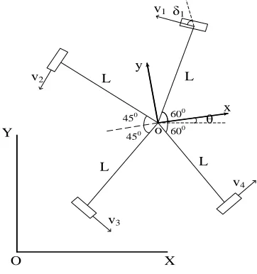
Because of the increase of shooting mechanism, those four omni-directional wheels of the soccer robot developed by our laboratory are not uniformity distributed. The angle between the two front wheels is 120
, and the angle between the two rear wheels is 90 . The kinetic model of this four-wheel omni-directional mobile robot is shown in Figure 1.
L
L L
L
600
600 450 450
v4
v3
v2
v1 δ1
θ x y
o
O Y
[image:2.612.326.522.138.195.2]X
Figure 1: Kinetic Model Of The Robot
According to the geometric relationship of Figure 1, the kinetic model of mobile robot can be constructed as follows:
1 1 1
2 2 2
3 3 3
4 4 4
sin( ) cos( )
sin( ) cos( )
sin( ) cos( )
sin( ) cos( )
v L
X
v L
Y
v L
v L
δ θ δ θ
δ θ δ θ
δ θ δ θ
θ
δ θ δ θ
− + +
− − − −
=
+ − +
− −
(1)
Where p=
(
X Y θ)
τ denotes the velocity at any time of the centroid, θ denotes the motion direction of robot, θ denotes the angular velocity ofrobot, the positive direction is anticlockwise; Each of v1,v2,v3 and v4 denotes the linear velocity of four wheels respectively. Each of δ1 , δ2 , δ3 and δ4
denotes the angle between wheel and x axis respectively, but δ2,δ3 and δ4 are not shown in Figure 1. Each value of δ1 , δ2 , δ3 and δ4 is
60 ,45 ,45 and 60 respectively. L denotes the distance between the center of car-body and the center of wheel.
2.2 Lateral Position Error Model Of Mobile Robot
Preview path
X Y
O
x y
v P
X(t) XP(t+T)
x(t) Y(t)
y(t)
θ
robot xP(t+T)
yP(t+T)
YP(t+T)
y(t)
[image:2.612.315.520.403.583.2]Preview point
Figure 2: Lateral Position Error Model Of The Robot
[image:2.612.104.285.505.698.2]relative coordinate system is ( x t( ) , y t( ) ), the directional angle of robot is θ.
The robot’s path function under absolute coordinate system can be expressed as: Y=Y X( ), and under the relative coordinate system, it can be expressed as y=y x( ) , the relationship between
( , )x y and (X Y, ) can be expressed as:
cos sin
cos sin
X x y
Y y x
θ θ
θ θ
= −
= +
(2)
In this way we can change the path function from absolute coordinate system to relative coordinate system according to the direction angle of robot θ on every moment.
Secondly, preview points are confirmed. According to the preview time denoted as T, it can
be confirmed that the preview point P in x-coordinate on relative coordinate system can be expressed as:
( ) ( ) ( )
P
x t+T =x t +Tx t (3)
According to the x-coordinate of preview point P
and path function y=y x( ), it is confirmed that the preview point’s y-coordinate on relative coordinate system can be expressed as:
[ ( )]
P P
y = y x t+T (4)
Meanwhile, the preview distance can be expressed as:
2 2
[ P( ) ( )] [ P( ) ( )]
d= x t −x t + y t −y t (5)
Finally, the lateral position error of robot is confirmed, at present time t, lateral position error can be expressed as:
( ) [ ( )] ( ) y t y x t y t
∆ = − (6)
And the lateral position error of robot with respect to preview point P is:
( ) [ ( )] ( ) ( )
P P
y t T y x t T y t T y t
∆ + = + − − (7)
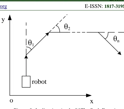
2.3 Curvature Of Preview Point For Robot For each point in path function Y=Y X( ) under the absolute coordinate system, the path function’s slope in this point can be confirmed. Using '
tan
[image:3.612.311.519.71.255.2]Y = θ to obtain each line-segment and its adjacent line-segments’ tilt angle error θ , θ is the motion direction angle of robot. Each point’s inclination angle of path function in a certain section is shown in Figure 3:
o
x
y
θ
nθ
2θ
1robot
Figure 3: Inclination Angle Of The Path Function
At time t, it is defined a preview point curvature
as 1 ( )
n
i
i
w t θ
=
=
∑
, n is the number of preview points.Considering driver can consider nearby road conditions, use the principle which called “near big, far small”, according to the preview point distance, the curvature of preview point is rewritten as:
1 ( )
n
i i
i
w t a θ
=
=
∑
(8)Where weight coefficient ai ≥0 and 1
1
n
i
i
a
= =
∑
.3
PREVIEW CONTROL OF THEFOUR-WHEEL OMNI-DIRECTIONAL MOBILE ROBOT
Because of the motion character of omni-directional mobile robot, the robot’s angular velocity can be designed individually, thus this paper only discusses the translational situation of the robot. From the analysis result of above section we can know that, assume the robot’s longitudinal position error is e k( ) when time is k, and the longitudinal
position error relative to preview point P is e kP( ). At this moment, the curvature of the path function is
( )
w k and the curvature of the preview point is w kP( ).
Based on different longitudinal position error and curvature, we choose different preview distance d, the number of preview point n , robot’s lateral velocity x t( ) and longitudinal velocity y t( )
The fuzzy controller chooses robot’s longitudinal position error and the real-time path curvature as input variable. The output variable include preview distance d, the number of preview point n, robot’s lateral velocity x t( ) and longitudinal velocity y t( ). The fuzzy statement of input output variable will be divided into 7 kinds, namely NB、NM、NS、ZO
、PS、PM、PB,and membership function is triangular function.
Each variable approximately obeys the following rules:
(a) If preview distance d is near, the predictability to trajectory changing is poor, and tracking failure will occur when the robot take a sudden turn. We choose d variable strategy, when
( )
P
w k is small, the trajectory variation is small, d should be increased properly, otherwise d
should be decreased.
(b) When the number of preview point n is fixed and the path camber is not so large, undesired signal will be brought in if n is large, which
will cause the motion direction angle of robot change frequently and deteriorate car-body stability. However, using n variable strategy, the larger w kP( ) is, the larger n is, thus
improve the predictability of controller.
(c) The robot will lose trajectory easily in big camber when lateral velocity x t( )is fixed, so
( )
x t variable strategy is adopted, as curvature
( )
P
w k becomes larger, x t( ) should be decreased appropriately, otherwise x t( ) will be increased.
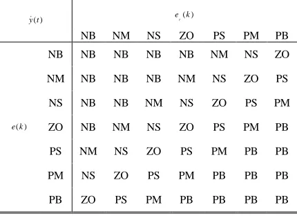
(d) Longitudinal velocity y t( ) is variable, it should be adjusted appropriately according to the change of e k( ) and e kP( ).
Thus, we can build specific control rules, as shown in TABLE I to TABLE IV.
Table I : Control Rules Of Preview Distances d
( )
P
w k NB NM NS ZO PS PM PB
d PB PM PS ZO NS NM NB
Table II : Control Rules Of The Number Of Preview Point n
( )
P
w k NB NM NS ZO PS PM PB
n NB NM NS ZO PS PM PB
Table III : Control Rules Of Lateral Velocity x t( )
( )
P
w k NB NM NS ZO PS PM PB
( )
[image:4.612.310.525.251.407.2]x t PB PM PS ZO NS NM NB
Table IV : Control Rules Of Longitudinal Velocity y t( )
( )
y t eP( )k
NB NM NS ZO PS PM PB
( ) e k
NB NB NB NB NB NM NS ZO
NM NB NB NB NM NS ZO PS
NS NB NB NM NS ZO PS PM
ZO NB NM NS ZO PS PM PB
PS NM NS ZO PS PM PB PB
PM NS ZO PS PM PB PB PB
PB ZO PS PM PB PB PB PB
4
SIMULATION AND ANALYSIS4.1 Simulation Platform And Environment This paper carry out the modeling and simulation analysis of robot’s motion control system based on Matlab7.0 environment, the motor’s performance parameters in simulation experiments are as follows: rated power is 60W, rated torque is 85mNm, rated speed is 8050rpm, rated voltage is 24V, rated current is 3.44A, rotor inertia is 33.3gcm2, armature resistance is 0.611 Ω, armature inductance is 0.119mH, torque constant is 25.9mNm/A, velocity constant is 369rpm/V, mechanical time constant is 3.03ms, motor reducer’s drive ratio is 1:22 and the moment of inertia is 0.8gcm2. The robot’s parameters are as follows: the quality is 23kg, the radius is 22.5cm, the wheel radius is 10cm, and the friction torque of single wheel is 1.86Nm.
4.2 Comparison And Analysis Of Experiment Results
path are chosen separately as the robot’s reference path to carry out the trace tracking experiment. During the experimental period, the Multi Points Preview Control (MPPC) method proposed in this paper is compared with the Fuzzy Control for Path Tracking (FCPT) method presented in [12]. The tracking results and errors are shown in Figure 4 to Figure 6.
0 1 2 3 4 5 6 7 8 9 10 11 12 13 14 15
-5 0 5 10 15 20 25 30 35 40
x/m
y
/m
Reference FCPT MPPC
(A) Curves Of Path Tracking
0 1 2 3 4 5 6 7 8 9 10
-2 -1 0 1 2
t/s
e/
m
Reference FCPT MPPC
[image:5.612.90.298.191.441.2](B) Curves Of Path Tracking Errors
Figure 4: Straight Path Tracking Results
From Figure 4, it can be seen that the robot exists large error during the whole track procedure employing the FCPT method due to the coupling characteristic between each wheel and the uncertainty of the system’s parameter, while adopting the MPPC method presented in this paper, the robot track tracing error is small, the time that the system achieve stable state is short. In the initial stage, the track tracing error is big owing to the robot’s high velocity changing. With the enhancement of controller action, the robot’s velocity gradually tends to stable and path tracking error reduced gradually.
0 1 2 3 4 5 6 7 8 9 10 11 12 13 14 15
-2 -1 0 1 2 3 4
x/m
y
/m
Reference FCPT MPPC
(A) Curves Of Path Tracking
0 1 2 3 4 5 6 7 8 9 10
-2 -1 0 1 2 3 4
t/s
e/
m
Reference FCPT MPPC
(B) Curves Of Path Tracking Errors
Figure 5: Sine Path Tracking Results
From Figure 5, we can see that when robot’s tracking path is curve, the robot path tracking effect is poorer using FCPT method and the tracking error is bigger, especially when path curvature changes greatly. Because the future path information is not considered, the tracking errors change very big, which will cause the path lose condition. While with MPPC method, the robot can preferable track reference path. Due to the controller contains path curvature information, the robot can still track the reference path better when the path changes a lot , and the whole tracking error of the robot is rather small either.
-2 -1.5 -1 -0.5 0 0.5 1 1.5 2 2.5 3 -2
-1.5 -1 -0.5 0 0.5 1 1.5 2
x/m
Reference FCPT MPPC
(A) Curves Of Path Tracking
0 1 2 3 4 5 6 7 8 9 10
-2 -1 0 1 2 3 4
t/s
e/
m
Reference FCPT MPPC
[image:5.612.263.514.388.693.2](B) Curves Of Path Tracking Errors
From Figure 6, the control output of FCPT method changes quickly due to the path curvature changes continuously when the robot track circular path in great change. Due to mechanical system exists friction, inertia etc factors, the robot can’t make a rapid response. The path tracking error is very large, which makes it difficult to achieve the ideal tracking effect. Because MPPC method can correct the robot’s motion velocity in time according to the curvature change of path and preview point information, thus reduce the tracking errors, ensure that when the robot path changes greatly, the robot can still realize fast tracking.
TABLE Ⅴ Comparison Of Maximum Error And Average
Error Under Different Path Tracking
Type of path Straight path
Sine path
Circula r path
Maximum-Error (m)
FCPT 0.55 1. 23 1.14
MPPC 0.27 0.35 0.42
Average-Error (m)
FCPT 0.31 0.74 0.58
MPPC 0.02 0.12 0.19
Table Ⅴ shows the maximum error and average error comparison when robot track different path using different method. From above figures and TableⅤ, it is known that the maximum error and the average error when tracking straight path are less than the other two kinds of path. It shows the best tracking effect. It is because that when tracking path curvature changes greatly or changes quickly, although the output of controller has changed, due to motion inertia cause robot system unable to change its velocity of movement in time, especially in the high velocity motion condition may cause a loss of robot reference path, even the robot will be out of control. So in the design of robot reference path, we should try to use the straight path to carry on the trajectory tracking.
5
CONCLUSIONThis paper discuss four-wheel Omni-direction mobile robot trajectory tracking problem, in view of the traditional control method, the robot’s tracking ability to the expected trajectory is poor, this paper presents the MPPC method. Firstly, the robot’s lateral position error model is established, and on this basis to determine the lateral position error and curvature size of the preview point. At the same time, the current position error and preview point position error are considered to design the fuzzy controller, according to the preliminary preview
information of different path, longitudinal velocity and lateral velocity of the robot are adjusted online to achieve the expected trajectory tracking. The experimental results show that when using the MPPC method for path tracking, the robot path tracking error is small, even if the tracking path changes bigger, it can also carry on the trajectory tracking fast, thus meets the tracking requirements under different path circumstance.
ACKNOWLEDGMENTS
The work of this paper is supported by the Natural Science Fund of Guangdong Province (No. S2011010004006), the Science and Technology Planning Project of Zhaoqing City (No. 2010F006, No. 2011F001), and the Research Initiation Fund of Zhaoqing University (No. 2012KQ01).
REFRENCES:
[1] M. J. Jung, H. S. Kim, S. Kim, et al, “Omni-directional mobile base OK-II”, Proceedings of the IEEE International Conference on Robotics and Automation, IEEE Conference Publishing Services, April 24-28, 2000, pp. 3449-3454.
[2] Y. F. Liu, Q. Li, S. Q. Jiang, et al, “The design and simulation of control system of omni-directional mobile robot", International Symposium on Intelligent Information Technology Application Workshops, IEEE Conference Publishing Services, December 21-22, 2008, pp. 147-150. [3] H. M. Feng, C. Y. Chen, J. H. Horng, “Intelligent
omni-directional vision-based mobile robot fuzzy systems design and implementation”, Expert Systems with Applications, Vol. 37, No. 5, 2010, pp. 4009-4019.
[4] M. C. Mickle, R. Huang, J. J. Zhu, “Unstable, nonminimum phase, nonlinear tracking by trajectory linearization control", Proceedings of the IEEE International Conference on Control Applications, IEEE Conference Publishing Services, September 2-4, 2004, pp. 812-818. [5] Y. Ueno, T. Ohno, K. Terashima, et al, “Novel
[image:6.612.93.296.276.372.2][6] S. Han, H. S. Lim, J. M. Lee, “An efficient localization scheme for a differential-driving mobile robot based on RFID system”, IEEE Transaction on Industrial Electronics, Vol. 54, No. 6, 2007, pp. 3362-3369.
[7] Y. Liu, J. J. Zhu, R. L. Williams, et al, “Omni-directional mobile robot controller based on trajectory linearization”, Robotics and Autonomous Systems, Vol. 56, No. 5, 2008, pp. 461-479.
[8] T. H. Liu, H. H. Hsu, “Adaptive controller design for a synchronous reluctance motor drive system with direct torque control”, IET Electric Power Applications, Vol.1, No. 5, 2007, pp. 815-824. [9] K. B. Kim, B. K. Kim, “A minimum-time
trajectory for three-wheeled omnidirectional mobile robots following a bounded-curvature path with a referenced heading profile”, IEEE Transactions on Robotics, Vol. 27, No. 4, 2011, pp. 800-808.
[10] S. H. Chen, J. C. Juang, S. H. Su, “Backstepping control with sum of squares design for omni-directional mobile robots”, Proceedings of ICROS-SICE International Joint Conference, IEEE Conference Publishing Services, August 18-21, 2009, pp. 545-550.
[11] D. Chwa, “Sliding-mode tracking control of nonholonomic wheeled mobile robots in polar coordinates”, IEEE Transactions on Control Systems Technology, Vol. 12, No. 4, 2004, pp. 637-644.
[12] T. L. Lee, L. C. Lai, C. J. Wu, “A fuzzy algorithm for navigation of mobile robots in unknown environments”, Proceedings of the IEEE International Symposium on Circuits and Systems, IEEE Conference Publishing Services, May 23-26, 2005, pp. 3039-3042.