ISSN: 1992-8645 www.jatit.org E-ISSN: 1817-3195
LATENCY AND ENERGY AWARE BACKBONE ROUTING
PROTOCOL FOR MANET
1P.FRANCIS ANTONY SELVI, 2M.S.K.MANIKANDAN
1
Department of Electronics and Communication Engineering R.V.S College of Engineering and Technology Dindigul, Tamil Nadu
2
Department of Electronics and Communication Engineering Thiagarajar College of Engineering, Madurai, Tamil Nadu E-mail: [email protected] , [email protected]
ABSTRACT
Earlier woks on latency reduction in mobile ad hoc network (MANET) routing, lead to huge energy consumption due to the heavy load on each mobile node. There is a trade-off between energy reduction and latency reduction. Moreover, existing latency reduction techniques rarely consider retransmission latency, queuing latency and MAC layer latency apart from routing latency. In this paper, we propose to design a latency and energy aware backbone routing protocol for MANET. In the proposed protocol, backbone nodes collect the information of Residual Energy, Delay, MAC contention and Load from the nodes using neighbor monitoring mechanism. The collected information is stored in the Local Topology table from which the best routing paths are selected using the backbones.
Keywords: Latency Reduction, MANET, Energy Consumption, MAC, Routing Protocol
1. INTRODUCTION
An ad hoc network can be formed on-the-fly and spontaneously without the required intervention of a centralized access point or an existing infrastructure. Applications of an ad hoc network include battlefield communications, emergency rescue missions and disaster recovery where the communication infrastructure is abolished. Further, people may communicate forming an ad hoc network in online conferences and classrooms. Thus, an ad hoc network may provide a cost-effective and cheaper way to share information among many mobile hosts. [1]. It is a network without any base stations infrastructure-less or multi-hop. [2] Large network latency affects all aspects of data communication in a MANET, including an increase in latency, packet loss, required processing power and memory. [4] Applications like Military Applications require Low Latency but Ad Hoc Networks suffer huge high latency. [6]
To maximize the Ad Hoc network lifetime we need to find a route which minimizes the amount of energy consumed. Most of the Ad Hoc network nodes are mobile in nature so it has limited battery power so there is a huge need to reduce energy consumption. [7] Since transmission of a single bit of data is equal to processing thousand operations in sensor processor. Using smart badges in applications like military or hotels consumes more energy. [8]
Applications like military requires its nodes to respond very quickly to any intrusion on detection if the sensor is out of energy then detection are not made.
2. RELATED WORKS
Abdel Ilah Alshabtat et al [9] proposed a new routing protocol for Unmanned Aerial Vehicles (UAVs) that equipped with directional antenna. They named this protocol Directional Optimized Link State Routing Protocol (DOLSR). This protocol is based on the well known protocol that is called Optimized Link State Routing Protocol (OLSR). They focused in our protocol on the multipoint relay (MPR) concept which is the most important feature of this protocol. They developed a heuristic that allows DOLSR protocol to minimize the number of the multipoint relays. With this new protocol the number of overhead packets will be reduced and the End-to-End latency of the network will also be minimized.
Malik, M.I. et al [11] have proposed a novel cross layer approach to mitigate the latency issues inherently present in the AODV at the same time maintaining the efficient use of battery power. They have used received Log-Likelihood ratios (LLR) at each node as the decisive parameter whether or not to participate in the transmission. The proposed LLR based approach adapts itself according to the nature of traffic. If there is real time traffic, the nodes operate at high transmission power and in case of non real time traffic the transmission power is low. Though [11] considers both latency and power, since node has to make the routing decision, the overhead will be more. Apart from this, the queuing and retransmission are delays are not considered.
Yangcheng Huang et al [12] have presented a fast neighbor detection scheme for proactive MANET routing protocol. Instead of using periodic HELLO messages, they have used explicit handshake mechanism to reduce the latency in neighbor detection. In particular, two route handshake options are presented, namely the Broadcast based handshake (BHS) algorithm and Unicast based handshake (UHS) algorithm. Though the neighbor detection mechanism of reduces routing delay, it does not consider the queuing, retransmission and maintenance delays.
Hanan Shpungin et al [13] have proposed Energy Efficient Online Routing in Wireless Ad Hoc Networks. In this paper they study the minimum total energy and maximum network lifetime routing problem in wireless ad hoc networks. They develop competitive online schemes for an infinite sequence of random routing requests with provable approximation factors in both measures. In addition, we produce fundamental bounds on the expected total energy consumption and network lifetime in the optimal offline solution.
3. PROPOSED METHODOLOGY
There is a need for technique which considers all the latencies along with reduced energy consumption. In this paper, we propose Latency and Energy Aware Backbone Routing (LEABR) to design a multipath routing backbone in MANET. In the proposed protocol, we construct a routing backbone for MANET with special types of nodes. It consists of 4 phases, namely Backbone construction, Neighbor Monitoring, Routing Decision and Route updating.
3.1 Overview
In this proposed protocol, we propose to design a multipath routing backbone for latency and energy reduction in MANET.
3.2 Estimating Parameters for Routing in MANET
3.2.1 Estimating Residual Energy
Transmission and reception causest energy consumption in a node, therefore Residual Energy is calculated after every Δ seconds. Assume d is the distance between nodes of packet size 1. [17-2]
RE of a node v is calculated based on upstream nodes (nu) and downstream nodes (nd) which are used for transmitting and receiving packets. Thus the energy required by node v to transmit packets of l units to its downstream nodes which are at a distance d is given by:
∑
= ∞ =
nd
i
i i T m
T E l d
E
1
) ,
( (1)
And the energy required by node x to receive packets of l units from its upstream nodes is given by:
∑
= ∞ ∞ =
nu
i i m
R ER l
E
1
)
(
(2)
The total energy consumed when multiple flows are considered is given by:
m o m R m T m
tot E E E
E
∞ ∞
∞ + +
= (3)
Where Emo∞ is the energy consumed in overhearing activities. Thus, the newly calculated residual energy when multiple flows are considered is calculated as:
m tot tot old m
new RE E
RE = −
(4)
3.2.2 Estimating Link Expiration Time
Path expiry can be determined based on the link expiry time. Link expiry time is the maximum time that two nodes remain connected. Motion parameters are considered to obtain link expiry time.
ISSN: 1992-8645 www.jatit.org E-ISSN: 1817-3195
λ
λ
λ
calculate d1 and d2 using the following formula:[18]
t
v
d
1
1
=
(5)t
v
d
2
2
=
(6))
cos
(
1
cos
1
1
1
1
x
'x
x
'd
1θ
1x
't
v
1θ
1x
=
+
=
+
=
+
(7)
)
sin
(
1
sin
1
1
1
1
y
'y
y
'd
1θ
1y
't
v
1θ
1y
=
+
=
+
=
+
(8) ) cos ( 2 cos 2 2 2
2 ' 2 2
2 2 '
' x x d θ x t v θ
x
x = + = + = +
(10)
)
sin
(
2
cos
2
2
2
2
y
'y
y
'd
2θ
2y
't
v
2θ
2y
=
+
=
+
=
+
(11) Distance D between two nodes at time t will be obtained from: 2 2 2 1 1 ' ' 2 2 2 1 1 ' ' )} sin sin ( ) 2 1 {( )} cos cos ( ) 2 1 {( θ θ θ θ v v t y y v v t x x D − + − + − + −
= (12)
When the distance between two nodes becomes larger than the transmission range the nodes will be disconnected. For transmission range r, Lept is the link expiry time between any two nodes overtime period t can be calculated by:
D r
Lept = (13)
Where Lept is the link expiry time.
3.2.3 Mobility Estimation
Mobility is estimated based power level at the destination node, d is the distance between source and destination pairs. Free space model is used in ideal situation, it is defined as the inverse square dependence of the ration of received power RxPr and transmit power TxPr on the distance between source and destination i.e. [19]
2 1 Pr Pr d α Tx Rx (13)
The above obtained expression cannot be suited for real life conditions where huge complexities are involved in estimating distance between source and destination in the case of accurate channel modeling. We can get a good knowledge of relative mobility between the two nodes based on the ratio of RxPr between two successive packet transmissions from neighboring nodes. Hence relative mobility, MrelY(X), at a node Y with respect to X, in this manner: old Y X new Y X rel Rx Rx X γ M → → = Pr Pr log 10 )
( 10
(14)
If RxPrnewX->Y < RxProldX->Y, then MrelY < 0, and a negative value of the relative mobility metric between any two nodes will indicate that the two nodes are moving away with respect to each other. On the other hand if RxPrnew > RxProld, then Mrel is positive, and that indicates that the nodes are moving closer to each other.
3.2.4 Estimating Delay
Delay is the amount of time taken for a packet to reach the destination. Delay is obtained from the sum of all the link delays. Clocks of all the mobiles are perfectly synchronized. [20]
The mean queuing delay which represents the interval between the time the packet enters in the queue of the link’s emitter and the time that the packet becomes the head of line packet in this node’s queue. They denote it by Dq. The mean contention delay is the interval between the time the packet arrives at the head of line and the time the packet is sent to the physical medium. They denote it by Dc. This interval reflects the fact that a node may contend to access to the channel because of other transmissions in its carrier sensing area. The mean transmission delay is the time to transmit the whole packet including possible retransmissions in case of collisions. They denote it by Dt.
Using IEEE 802.11, the mean packet delay PD
can be estimated as
t c
q D D
D
PD= + + (15)
3.2.4.1 Estimating the mean queuing and contention delay
μ λIn this case we consider two parameters and which indicates number of packets arriving at the queue per second and the number of packets leaving the queue per second.
We estimate the value of Dc + Dq in this section.
When μ > , the service rate that of the node is higher than the arriving process and there will be no accumulation in the queue involving a queuing and a contention delay which are null.
0 = + ⇒ > c q D D λ μ
When μ <= . Let’s denote by p (n) the probability to have n packets in the queue (n <= K). A packet arrives with rate and exits with rate μ. So:
) 0 ( * )
(n ρ p
p μ λ ρ n = ⇒ = Using
ρThe sum of the probabilities being equal to 1,
we can simply express p (n) in function of and K:
1 ≠ ρ + − − = + 1 1 1 1 ) ( 1 K ρ ρ ρ n p k n If 1 = ρ
The mean number of packets Q in the queue is therefore:
∑
= = K n n p n Q 0 ) ( *Using queuing theory and according to Little’s law, the parameter Dq + Dc is equal to the mean waiting time:
λ Q D Dq+ c =
So the final expression is:
1 ≠ ρ − + + − − = + + λ K λ ρ ρ K ρ K ρ ρ D D K K K c q 2 1 1 ) 1 ( 1 1 1 If 1 = ρ If
We can also notice that, since the queue size is bounded, equation editor Dq + Dc is bounded by a maximum value Dmax such as:
) (
lim
max q c
ρ
D D
D = +
+∞ → λ ρ ρ K D K K * * 1 2 max + + ≈ μ ρ
λ= * As
We have:
μ K
Dmax ≈ (16)
In this estimation, the contention delay only considers the time spent until the medium is free in order to gain the access to the radio medium to send the packet for the first time. We do not consider here the time that may be required to retransmit the packet.
3.2.4.2 Estimating Transmission Delay
The total time to transmit the whole packet on the medium is called as transmission delay. On success of this operation a positive ACK is sent it to the emitter. However, there is a maximum chance that single frame is emitted and the channel is not idle which results in collisions. These collisions will result in increase of CW and retransmissions with the increase in the mean transmission delay.
Back off is estimated using:
− + + − − − = p p p CW p p p backoff C c c 1 * * 2 1 ) * 2 ( 1 2 1 max
The different points mentioned above can be combined to estimate the mean transmission delay on a wireless link, i.e. between an emitter and a receiver. To summarize, the mean transmission delay between two neighbor nodes can be estimated by the following formula:
∑
− = + + = 1 0 * n k n c slott backoff T T T
D
m c slot
t backoff T n T T
D = * + * + (17)
Where Tc is the time to successfully transmit a whole packet of m bytes with IEEE 802.11, Tc is the collision duration; n is the mean number of retransmissions depending on collision probability, backoff is the expected number of backoff slots and Tslot is the duration of the slot.
To sum up, the mean delay D of a one-hop link consists of:
• The mean delay experienced by a packet on the link’s emitter (= Dq + Dc). It corresponds to the waiting time before the first transmission of the packet.
• The mean delay experienced by a packet during the transmission (= Dt). It includes the potential retransmissions induced by collisions.
3.2.5 Estimating MAC Contention
MAC has distributed coordination function (DCF) which has packet sequence as request-to-send
(RTS), clear-to-send (CTS), data and
ISSN: 1992-8645 www.jatit.org E-ISSN: 1817-3195
acc SIFS CTS RTS
occ t t t t
C = + +3 + (18)
Where tRTSand tCTSare the time consumed on RTS
and CTS, respectively and tSIFS is the SIFS period. Tacc is the time taken due to access contention.The
channel occupation is mainly dependent upon the medium access contention, and the number of packet collisions. That is, Cocc is strongly related to the
congestion around a given node. Cocc can become
relatively large if congestion is incurred and not controlled, and it can dramatically decrease the capacity of a congested link.
3.2.6 Estimating Traffic Load
If we measure the inter-arrival time between two packets, say Δt seconds, and size of packet, say ΔL
bits. Then the traffic load through the node, say Lest
is given in (19):
onds bits
t L Lest
sec ) (
∆ ∆
= (19)
Another way is to take time average over time, sayTws.This is shown in (20):
onds Packets n
T L
ws est
sec * ) 1 (
= (20)
Where Lestis the estimated traffic load through the
node, n is the number of packets that have arrived in
the time Tws. A design parameter here is the time Tws
. We will call it the window size. [22]
3.3 Construction of Routing Backbone in MANET
Routing backbone construction in MANET consists of the following 4 phases: Backbone Construction, Neighbor Monitoring, Routing Decision and Route Updating.
3.3.1 Backbone Construction
We propose an efficient algorithm to construct a strong and small virtual backbone.
During the execution of the algorithm, distributed coloring process is used to color nodes in the network with three colors: black, gray, and red. After the execution of the algorithm, the node will be marked black, red, or gray. All black nodes compose a Large Independent Set (LIS) of the network; all red nodes are the nodes connecting the LIS into a virtual backbone. Thus all black nodes and red nodes compose the virtual backbone. All gray nodes are dominates.
(i) Node Ranking
Node ranking is used for a node to decide whether it is an initiator and for breaking ties when two candidate nodes can be chosen into the backbone, or two candidate nodes can be chosen as the connectors. We define the node ranking is a tuple of (Residual Energy (RE), Link Expiration Time (LET), Mobility (M)) of a node. Stability is for measuring mobility and effective degree is for estimating the coverage of a node. For a white node, effective degree is the number of its white neighbors. For nodes with other colors, effective degree is its degree. A node v is of greater rank than other node u if:
1. REv > REu or
2. REv = REu and LETv > LETu or
3. REv = REu and LETv = LETu and Mv < Mu The stability of each node can be estimated using its previous location information since there is usually temporal and spatial locality in node movement.
Clearly, the more a node moves, the less stability it has.
(ii) Forest Construction
A forest consists of multiple trees. Starting from multiple initiators, multiple dominating trees composing the forest are constructed in parallel [16].
To distinguish different dominating trees, we introduce two terms
(i) Parent of a node u: the node which is in the same dominating tree as u and decides the u’s color;
(ii) Root of a node u: The initiator of
(iii) the dominating tree where u belongs. Note that every node has only one root and one parent.
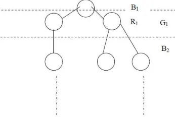
Each gray node in Gi must have at least one neighbor in Bi and 0 or more neighbors in Bi. Each black node in Bi must have at least one gray neighbor in Gi, thus it is guaranteed to be Gi able to find gray nodes in to connect Bi nodes to Bi nodes. In Figure. 1, we already know that every G1 node is connected to the B1 node which is the initiator, thus we can guarantee to form a tree (thick lines and nodes in the figure) using our algorithm. We call this tree dominating tree. Note that the leaves of the dominating tree can only be black or gray, but could not be red. Gray nodes can only be leave nodes. Every node records its parent information during the coloring process to maintain the tree structure R1 in Figure. 1 represents connectors at the 1st round.
Figure.1. Inter Connecting Backbone Nodes
The dominating tree construction algorithm is described in Algorithm 1. Each node calculates its own rank as described in Section 1. Each node maintains its parent and root information and gray nodes keep a list of black neighbors.
There are five types of messages: black, gray, black-to-be, red, and connect. The first four are for a node to announce its own status, connect message is for a black node to choose a gray neighbor as connector. The formats of the messages are defined as follows:
1. Black: black, M, stability, degree, root M. 2. Black to be: black to be M, stability, effective
degree, parent M, root M.
3. Gray: gray, id, stability, degree, parent M, root M
4. Red: red, M, stability, list of Black Neighbors 5. Connect: connect, M
Algorithm 1
1: Initially: The white node with highest rank among its one-hop neighborhood;
2: Initiator turns into black and broadcasts black message;
3: If (a white node u receives black messages) Then
u turns into gray and broadcasts gray message; End if
4: If (a white node u receives gray messages) Then
u broadcasts black to be message; End if
5: If (a white node u has broadcasted black to be message)
Then
If (u receives black message) Then
u turns into gray and broadcasts gray message;
End if
6: If (u has the highest rank among the senders of blacktobe messages it received or all its neighbors with higher ranks which have sent blacktobe message have turned gray)
Then
u turns into black and broadcasts black message;
u picks its gray neighbor with highest rank and unicast connect message to the gray node;
End if End if
7: If (a gray node u receives connect message) Then
u turns into red and broadcasts red message;
End if
3.3.2 Neighbor Monitoring
In this phase, the backbone observes and collects the following information from its neighbors:
1. Residual Energy
2. Delay
3. MAC contention
4. Load
The above parameters are estimated as per the sections 3.2.1, 3.2.4, 3.2.5 and 3.2.6.
1. The backbone node is the core node in this network such that it performs routing the data from source node to destination node.
2. To perform routing the backbone node should know the status of its neighboring nodes which is obtained by sending PREQ (Parameter Request) to its 1-hop neighboring nodes after every Δ sec.
ISSN: 1992-8645 www.jatit.org E-ISSN: 1817-3195
4. The estimated parameters are put into PREP packet and sent to backbone node.
5. The backbone node will store the estimated parameters in the Local Topology Table (LCT).
[image:7.595.85.526.84.554.2]6. In order to route the data from a given source node to destination node, the LCT should be given to other backbone nodes. Hence the LCT will be routed to other backbone nodes.
Figure.2. Neighbor Monitoring
Figure 2 describes the neighbor monitoring mechanism by the backbone nodes. Initially, the Neighbor Backbone (NB) node 1 sends PREQ to the near by node A, then node A estimates the values (RE, LAT, TD, and MAC) and send backs PREP to the NB node 1. BB node 1 will tabulate the values and put into ICT and distribute ICT to other BB nodes.
3.3.3 Routing Decision Algorithm 2
1. If (Node S needs to send data to D) Then
RREQ is sent to NBB node // NBB: Nearest Backbone Node
End If
2. Next, the NBB node will select the best intermediate node of S based on the values of Latency, MAC contention, load and Residual energy.
3. While (IN not selected) // IN:
Intermediate Node {
If ((INLAT <ThLAT) && (INRE > ThRE) && (INLD < ThLD) && (INMAC < ThMAC))
Then IN is selected Else
IN is not selected End If
}
4. The selected IN’s information will be sent to the next BB node until it reaches destination’s NBB node.
5. Next, the RREP will be sent to the source node S via the Intermediate backbone node where the RREP consists of best path for the transmission of data from node S to node D.
[image:7.595.99.270.242.492.2] [image:7.595.324.498.333.568.2]node A. The computed path is used by the node A to send data to the node B.
3.3.4 Route Updating
Since the nodes are mobile, LCT will not be consistent throughout the life time of the network. Hence the BACKBONE nodes have to periodically monitor the neighboring nodes for updating the LCT. The updated LCT is again transmitted to other backbone nodes through the dedicated path
4. SIMULATION RESULTS
4.1 Simulation Model and Parameters
We use NS2 [24] to simulate our proposed Latency and Energy Aware Backbone Routing (LEABR) Protocol. In this simulation, the channel capacity of mobile hosts is set to the same value: 2 Mbps. The distributed coordination function (DCF) of IEEE 802.11 for wireless LANs is used as the MAC layer protocol. It has the functionality to notify the network layer about link breakage.
In this simulation, mobile number of mobile nodes is 50 moves in a 1500 meter x 300 meter rectangular region for 50 seconds simulation time. We assume each node moves independently with the same average speed. All nodes have the same transmission range of 250 meters. In our simulation, the speed is 5 m/s. The simulated traffic is Constant Bit Rate (CBR).
Our simulation settings and parameters are summarized in table 1
Table1 Simulation Parameters No. of Nodes 50
Area Size 1500 X 300
Mac 802.11
Radio Range 250m Simulation Time 50 sec Traffic Source CBR Packet Size 512
Mobility Model Random Way Point
Speed 5m/s
Pause time 0,10,20,30 and 40 s
Rate 250Kb
Flows 1,2,3,4 and 5
4.2 Performance Metrics
We compare our LEABR protocol with the MCMIS [16] protocol. We evaluate mainly the performance according to the following metrics. Packet Drop, Average end-to-end delay, Average Packet Delivery Ratio, Throughput and Average Energy consumption.
4.3 Simulation Results
A. Varying No. Of Flows
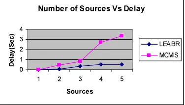
Initially, the performance of the protocols is measured by varying the no. of flows as 1,2,3,4 and 5.
Number of Sources Vs Delay
0 1 2 3 4
1 2 3 4 5
Sources
D
e
la
y
(S
e
c
)
[image:8.595.319.507.192.299.2]LEABR MCMIS
Figure 4: Flows Vs Delay
Figure 4 shows the delay occurred for both the protocols when the number of flows is increased. When the flows are increased, it leads more queuing delay and hence the end-to-end delay is also increased. From the figure, we can see that the delay of LEABR is 79% less than the existing MCMIS protocol.
Number of Source Vs Packet DeliveryRatio
0 0.5 1 1.5
1 2 3 4 5
Sour ces
D
e
li
v
e
ryR
a
ti
o
[image:8.595.105.279.515.645.2]LEABR MCMIS
Figure 5: Flows Vs Delivery Ratio
Figure 5 shows the packet delivery ratio for both the protocols when the number of flows is increased. The figure shows that the delivery ratio is same for both the protocols upto 3 flows and beyond that MCMS tend to decrease. From the figure, we can see that the delivery ratio of LEABR is 8% higher than the existing MCMIS protocol.
Number of Sources Vs Packet Drop
0 500 1000 1500
1 2 3 4 5
Sources
p
k
ts LEABR
[image:8.595.320.507.627.730.2]MCMIS
ISSN: 1992-8645 www.jatit.org E-ISSN: 1817-3195
Figure 6 shows the packet drop occurred for both the protocols when the number of flows is increased. The figure shows that there is no packet drop for both the protocols upto 2 flows and beyond that, the packet drop is increasing. From the figure, we can see that the packet drop of LEABR is 14% less than MCMIS.
Number of Sources Vs Energy Consumption
0 2 4
1 2 3 4 5
Sources
E
n
e
rg
y
(J
)
LEABR
MCMIS
Figure 7: Flows Vs Energy Consumption
Figure 7 shows the average energy consumption for both the protocols when the number of flows is increased. The figure shows that increase in number of flows has no impact on the energy consumption. But we can see that the energy consumption of LEABR is 24% less than MCMIS.
B. Based on Pause time
Next, the pause time of the nodes is varied as 0,10,20,30 and 40 seconds.
Pausetim e Vs Delay
0 1 2 3 4
0 10 20 30 40
Pausetim e(Sec)
De
la
y
(S
e
c
)
LEABR
MCMIS
Figure 8: Pause Time Vs Delay
Figure 8 shows the delay occurred for both the protocols when the pause time is increased. From the figure, we can see that the delay of LEABR is 84% less than MCMIS.
Pausetime Vs Packet Delivery Ratio
0 0.2 0.4 0.6 0.8 1
0 10 20 30 40
Pausetim e(Sec)
D
e
li
v
e
ry
Ra
ti
o
LEABR MCMIS
Figure 9: Pause Time Vs Delivery Ratio
Figure 9 shows the packet delivery ratio attained by both the protocols when the pause time is increased. From the figure, we can see that the delivery ratio of LEABR is 25% higher than MCMIS.
Pausetime Vs Packet Drop
0 500 1000 1500
0 10 20 30 40
Pausetim e(Sec)
P
k
ts LEABR
MCMIS
Figure 10: Pause Time Vs Drop
Figure 10 shows the packet drop occurred for both the protocols when the pause time is increased. From the figure, we can see that the packet drop of LEABR is 32% less than MCMIS.
Pausetime Vs Energy Consumption
0 1 2 3 4
0 10 20 30 40
Pausetim e(Sec)
E
n
e
rg
y
(J
)
LEABR MCMIS
Figure 11: Pause time Vs Energy
Figure 11 shows the average energy consumption for both the protocols when the pause time is increased. From the figure, we can see that the energy consumption MBRLER is 25% less than the existing MCMIS protocol.
5. CONCLUSION
MANET. In the proposed protocol, we have constructed a routing backbone for MANET with special types of nodes. It consists of 4 phases,
namely Backbone construction, Neighbor
Monitoring, Routing Decision and Route updating. The backbone observes and collects the following information from its neighbors: Residual Energy, Delay, MAC contention and Load. In the third phase, we choose the best path on the list of existing paths and finally in the fourth phase since the nodes are mobile, LCT will not be consistent throughout the life time of the network. Hence the BACKBONE nodes have to periodically monitor the neighboring nodes for updating the LCT. The updated LCT is again transmitted to other backbone nodes through the dedicated path.
REFERENCES:
[1] Ash Mohammad Abbas and Øivind Kure “Quality of Service in mobile ad hoc networks: a survey”, International Journal of Ad Hoc and Ubiquitous Computing, Volume 6 Issue 2, July 2010, Pages 75-98
[3] Ashwani Kush, Divya Sharma and Sunil Taneja, “A Secure and Power Efficient Routing Scheme for Ad Hoc Networks”, International Journal of Computer Applications (0975 – 8887) Volume 21– No.6, May 2011
[4] Nima Sarshar, Behnam A. Rezaei and Vwani P. Roychowdhury, “Low Latency Wireless Ad-Hoc Networking: Power and Bandwidth Challenges and a Hierarchical Solution”, Cornell University Library, arXiv:cs/0604021, 6 April 2006
[5] Wei-ping Shang, Peng-junWan and Xiao-dong Hu, “Improved Algorithm for Broadcast Scheduling of Minimal Latency in Wireless Ad Hoc Networks”, Acta Mathematicae Applicatae Sinica, English Series, Vol. 26, No. 1 (2010) 13– 22
[6] Josiane Nzouonta, Teunis Ott, Cristian Borcea, “Impact of Queuing Discipline on Packet Delivery Latency in Ad Hoc Networks”, Elsevier, Science Publishers, Volume 66 Issue 12, December, 2009
[7] Jinhua Zhu and Xin Wang, “A Progressive Energy Efficient Routing Protocol for Wireless Ad Hoc Networks”, INFOCOM 2005. 24th Annual Joint Conference of the IEEE Computer and Communications Societies. Proceedings IEEE 2005
[8] Gil Zussman and Adrian Segall, “Energy Efficient Routing in Ad Hoc Disaster Recovery Networks”, IEEE INFOCOM 2003
[9] Abdel Ilah Alshabtat, Liang Dong, “Low Latency Routing Algorithm for Unmanned
Aerial Vehicles Ad-Hoc Networks”, World Academy of Science, Engineering and Technology 80 2011 [10] Wei Wang, Student Member, IEEE, and
Boon-Hee Soong, Senior Member, IEEE, “Collision-Free and Low-Latency Scheduling Algorithm for Broadcast Operation in Wireless Ad Hoc
Networks”, IEEE COMMUNICATIONS
LETTERS, VOL. 11, NO. 10, OCTOBER 2007 [11] Malik, M.I, Shen Ting Zhi and Farooq, U,
”Latency aware routing mechanism to maximize the life time of MANETs” , International Conference on Computer Science and Network Technology (ICCSNT), IEEE 2011
[12] Yangcheng Huang, Bhatti, S and Sorensen, S.A,” Reducing Neighbor Detection Latency in OLSR”, IEEE 18th International Symposium on
Personal, Indoor and Mobile Radio
Communications, 2007. PIMRC 2007.
[13] Hanan Shpungin, “Energy Efficient Online Routing in Wireless Ad Hoc Networks”, Sensor, Mesh and Ad Hoc Communications and Networks (SECON), 2011 8th Annual IEEE Communications Society Conference on 2007. [14] Imrich Chlamtac a, Marco Conti b,*, Jennifer
J.-N. Liu, “Mobile ad hoc networking: imperatives and challenges”, ElseVier- Ad Hoc Networks 1 (2003).
[15] Deying Li a,b, Qin Liu c, Xiaodong Hu d, Xiaohua Jia, “Energy efficient multicast routing in ad hoc wireless networks”, ElseVier- Computer Communications 30 (2007) 3746– 3756
[16] Feng Wang, “On the Construction of Stable Virtual Backbones in Mobile Ad-Hoc Networks”, IEEE Transactions on Wireless Communications, Volume 8 Issue 3, March 2009, Pages 1230-1237
[17] Dilip Kumar S.M, and Vijaya Kumar B.P, “EAAC: Energy-Aware Admission Control Scheme for Ad Hoc Networks”, World Academy of Science, Engineering and Technology 27 2009.
[18] Md. Mamun-Or-RashidO and Choong Seon Hong, “LSLP: Link Stability and Lifetime Prediction Based QoS Aware Routing for MANET”, Korean Research Foundation 2006. [19] P. Basu, N. Khan, and T.D.C. Little, “A
ISSN: 1992-8645 www.jatit.org E-ISSN: 1817-3195
[20] Shreyas Prasad, Andr´e Schumache, Harri Haanp¨a¨a, and Pekka Orponen, “Balanced Multipath Source Routing”, 2007.
[21] S.Venkatasubramanian and Dr.N.P.Gopalan, “A QoS-Based Robust Multipath Routing Protocol for Mobile Adhoc Networks”, IACSIT International Journal of Engineering and Technology Vol.1,No.5,December,2009. [22] Seyed Hossein Kamali, “Traffic-Sensitive
S-TDMA Schedule Based on Traffic Load Estimate for Maintenance Self-Organized Radio Wireless Network”, 2008.