Analysis of the PROFIBUS Token Passing Protocol over Error Prone Links

(1)

A

NALYSIS OF THE

PROFIBUS T

OKEN

P

ASSING

P

ROTOCOL OVER

E

RROR

P

RONE

L

INKS

Andreas Willig

Technical University Berlin, Telecommunication Networks Group

Sekr. FT 5-2, Einsteinufer 25, 10587 Berlin, Germany

email: [email protected], phone: 49 30 31423818, fax: 49 30 31422514

June 9, 2003

Abstract

In this paper we investigate the properties of the PROFIBUS MAC protocol when operated over error prone links, like wireless links. In order to show that the protocol is very sensible to loss of control frames (e.g. token frames) we evaluate three performance measures, using a simulation approach: the mean delay, the mean station outage time and the cumulated outage time, i.e. the fraction of time where a single station is not member of the ring due to loss or error of control frames. The results indicate that the PROFIBUS MAC protocol is not really a good choice for use over error prone links.

I INTRODUCTION

The PROFIBUS is a widely used and well standard-ized field bus (german standard DIN 19245, see [2]). It is mainly used in industrial environments for applica-tions like interconnection of industrial controllers (PLC, CNC, RC), coupling of sensors and actors to a con-troller and so forth (distributed control applications). It is designed to meet some hard real time requirements for industrial communication purposes. As transmis-sion medium shielded twisted pair or fibre optic cables can be used. However, during the last years there was rapidly growing interest in wireless technology. Making the different benefits of wireless technology available for PROFIBUS installations has some advantages: stations can be attached and (re-)moved easily without changing a cabling system, stations can be mobile, switching from PROFIBUS LAN to PROFIBUS LAN or moving within a single PROFIBUS LAN and furthermore, when using a wireless link there is no cable which can be damaged or destroyed, thus there are less opportunities for break-downs of a production plant.

Our current research effort aims at the definition of a wireless extension to wired PROFIBUS with the final goal of joint operation of wired and wireless parts within a single LAN. One important question is, whether it is possible or desirable to use the PROFIBUS MAC proto-col (which uses token passing similar to IEEE 802.4) on top of a wireless medium or better to use something else.

So it is natural to ask, how the token passing protocol behaves on wireless links. Unfortunately, the character-istics of wireless technology are different from most of the cable types used in wired LANs. First, they tend to exhibit a nonstationary and bursty error behaviour, with very high bit error rates during an error burst. Second, due to the path loss it may happen that not all stations hear each other, i.e. we have only partial reachability. For these reasons one cannot expect the same behaviour of the PROFIBUS MAC protocol on a wireless link as on a wired link.

When considering transmission over an error prone and lossy medium, performance degradations mainly stem from two sources: one source is the loss of data frames, making retransmissions necessary, the other source is the vulnerability of the additional protocol mechanisms and frame formats used. The main ques-tion is, how the loss of special control frames affects the performance as compared to the case where there is no loss of special frames or where the protocol does not use special frames at all.

In this paper we analyze the behaviour and perfor-mance of the PROFIBUS MAC protocol when operated over error prone links in a case, where all stations can hear each other (fully meshed topology)1, using a simu-lation approach. We show that the special control pack-ets used for token passing and ring maintenance make the protocol vulnerable for serious performance

(2)

dations if the link exhibits a high error rate. As perfor-mance measures we use the mean delay for user data, the mean station outage time (i.e. the mean duration needed to re-include a station in the ring after it gets lost) and the cumulated station outage times.

The paper is structured as follows: in section II we describe the important characteristics of the PROFIBUS token passing protocol, in section III we describe the two basic error models used in our simulations, while in sec-tion IV we present our performance metrics, the simu-lation scenarios and the simusimu-lation results. Finally, in section V our conclusions are given.

This paper is a shortened version of a technical re-port [9]. Due to lack of space we discuss only the protocol behaviour. In the report we additionally ana-lyze the frame formats and error detection capabilities of PROFIUS, showing that these are not designed for er-ror prone links. Furthermore, we propose and analyze two slight changes to the protocol, which improve the performance of the protocol significantly, while not ne-cessitating changes in the protocol or frame formats.

II OVERVIEW ON THEPROFIBUS TOKEN

PASSINGPROTOCOL

The PROFIBUS is standardized in [2], with some corrections in [7]. It comes in different “flavors”. One of them (PROFIBUS-FMS) is intended for use on the cell level in a factory, having multiple active stations (see be-low). In this paper we focus solely on PROFIBUS-FMS. The PROFIBUS uses two different protocol ap-proaches on the MAC layer: a master/slave protocol for exchange of data frames (or “telegrams”) and a to-ken passing protocol for managing the case of multiple masters. The token passing protocol uses a broadcast medium. A logical ring is formed by ascending station addresses. The address space is small, a station address is in the range of 0 to 126, only a single octet is used for addresses. Every station (denoted as TS: This Station) knows the address of its logical successor (NS: Next Station) and its logical predecessor (PS: Previous Sta-tion). This knowledge is obtained from the ring main-tenance mechanisms described below. If TS receives a token frame (with TS as destination address), it checks whether it was sent by its PS. If so, the token is accepted, otherwise the token frame is discarded. In the latter case, if the same token frame is received again as the very next frame, the token is accepted and the token sender is reg-istered as new PS. In any case after accepting the token TS determines its token holding time (THT) and sends its own data during the THT. After finishing, TS tries to pass the token to NS. On this behalf a token frame is sent to NS. After that TS listens on the medium for some activity. This can be reception of a valid frame header (indicating that NS has accepted the token) or reception of some erroneous transmission. However, TS listens on

the medium only for a short time (called slot time) which is typically chosen very sharp, e.g. in the range of 100

µsec to 400µsec, and is also used as timeout value for immediate acknowledgements. If this time passes with-out any bus activity the token frame is repeated. If there is again no activity, NS is assumed to be dead and TS determines the next station in the ring (i.e. the successor of NS), makes this the new NS and tries to pass the token to it, following the same rules. The new station can be determined from information gathered during ring main-tenance (LAS), see below. If TS finds no other station, it sends a token frame to itself. A special requirement is the following: TS must read back from the medium all token frames it transmits (“hearback”), in order to de-tect a defective transceiver and to resolve collisions (see below). If TS encounters a difference the first time, it behaves as after a correct token frame, i.e. it waits for some response. If there is no activity on the medium it repeats the token frame. If TS again encounters a dif-ference, it discards the token immediately and removes itself from the ring, behaving as newly switched on and “forgetting” all knowledge previously obtained.

If TS is newly switched on, it is required to first lis-ten passively on the medium, until it has received two successive identical token cycles. During this time it is not allowed to send or answer to data frames or to accept the token. Every station address found in a token frame belonging to this two cycles is included into a locally maintained list of active stations (LAS). After that TS can enter the ring if it is included by its predecessor. In addition, TS is required to maintain its LAS by inspect-ing every received token frame. A special rule in this maintenance process is the following: if TS is already included in the logical ring and founds itself “skipped” by a token frame (i.e. the address of TS lies within the address range spanned by sender and receiver of the to-ken frame) it removes itself from the ring and behaves as newly switched on.

(3)

[image:3.595.325.531.81.158.2]

Table 1: Parameters for Gilbert/Elliot channel model

Mean-BER = 0.001 Mean-BER = 0.0001

tb 0.0244 0.0144

tg 0.0617 0.0944

Eb 0.0036 0.00064

[image:3.595.86.291.87.152.2]

Eg 0.000082 0.00002

Table 2: Fixed Parameters for all simulations

Parameter Value

Bitrate 500 kBit/sec

Slot-Time 400µsec

Max. Number of Retransmissions 3 Number of Active Stations 4 Number of Passive Stations 1

station in GAPL responds as “ready” TS will change its NS, shorten its GAPL, update its LAS and then sends a token frame to the new station.

The period for scanning the GAPL is created by a special timer (“gap timer”), which is set as an integral multiple (“gap factor”, the standard requires values be-tween 1 and 100) of the TTRT. Adjusting this timer is a critical parameter for the delay necessary to (re-) include a station. If the period is short, bandwidth is wasted, if it is long then ring inclusion delays get larger.

A special mechanism is used for the very first ring initialization or for token loss due to system crash of the current token owner: every station listens permanently on the bus. If there is no bus activity for some time (the corresponding timer is called timeout timer), the station “claims the token”, i.e. it starts transmitting either data or a token frame. The timeout value is linearly depen-dent on the stations address2_.

In the PROFIBUS a distinction is made between ac-tive stations and passive stations. Acac-tive stations are ca-pable of participating in the token passing process, thus they get the token from time to time and take the role of a master station, performing some data transmission. A passive station cannot handle the token. In all cases it acts only as a slave, i.e. it responds only to request telegrams.

III CHANNELMODELS FORWIRELESSLANS

When studying protocol behaviour over wireless channels, some kind of channel error model is needed. In this work we consider radio transmission, e.g. using the license free 2.4 GHz ISM band (Industrial, Scientific and Medical band). It is widely accepted, that the ra-dio channel is a bad channel with non-stationary error characteristics, e.g. under Rayleigh fading exhibiting bit error rates of≈ 10−2_...10−3_{. The error process is}

constituted by phenomena like slow fading, fast fading, noise, delay spread, interference and a path loss which is quadratic or even worse in the distance between two stations. It is known that the error process often exhibits a bursty behaviour [6].

For modeling the error characteristics of a

wire-less channel on a high level (as compared to ray-tracing channel simulations) we use two different mod-els throughout this paper. The first is the simple “in-dependent” model, where bit errors occur independent from each other according to a predefined fixed bit er-ror rate (BER). This model is simple, but it is not ca-pable of capturing the bursty error characteristics of wireless LANs. The second model is the widely used “Gilbert/Elliot model” (here simply denoted as Gilbert model) [3], [1], [8]: the channel state is modulated ac-cording to a two state continuous markov chain with the states named Good and Bad (with mean duration of be-ing in state good or bad oftgortb respectively). Every state is assigned a specific constant bit error rate (BER),

Eg in the good state,Eb in the bad state (Eg Eb). Within one state bit errors are assumed to be indepen-dent. The bit error rates in general depend on the fre-quency and coding scheme used and on environmental conditions. When the error model is aimed to be realistic then between every pair of stations a separate channel is needed. These channels are in general not synchronous, but some correlations may be present e.g. due to inter-ference. However, in order to keep computational com-plexity low we use only a single channel for all stations. For our simulations, we have used the methodol-ogy given in [8] in order to derive the parameters for the markov chain according to the PROFIBUS physi-cal characteristics for two different mean bit error rates (MBER). These parameters are shown in table 1. They are used throughout this paper.

IV SIMULATIONRESULTS

In this section we define our performance measures of interest, describe the simulation scenarios and present our results. We are only interested in the case that there is more than one active station. In this paper, due to lack of space we look only at the following performance measures:

• Mean station outage time (i.e. the time necessary for re-including a lost station into the ring)

• Fraction of time that a station is in the ring

2_{This timeout timer is one of the reasons for introduction of the hearback feature: it is necessary in order to resolve collisions, which may occur}

(4)

0 0.2 0.4 0.6 0.8 1 1.2 1.4

5 10 15 20 25 30 35 40 45 50

MSOT (sec)

Gap Factor

Station 65

0 0.2 0.4 0.6 0.8 1 1.2 1.4

5 10 15 20 25 30 35 40 45 50

MSOT (sec)

Gap Factor

Station 65 Station 22

0 0.2 0.4 0.6 0.8 1 1.2 1.4

5 10 15 20 25 30 35 40 45 50

MSOT (sec)

Gap Factor

Station 65 Station 22 Station 39

0 0.2 0.4 0.6 0.8 1 1.2 1.4

5 10 15 20 25 30 35 40 45 50

MSOT (sec)

Gap Factor

Station 65 Station 22 Station 39 Station 69

0 0.2 0.4 0.6 0.8 1 1.2 1.4

5 10 15 20 25 30 35 40 45 50

MSOT (sec)

Gap Factor

[image:4.595.99.283.53.188.2]

Fig. 1: MSOT vs. gap factor (Indep. Errors)

0 0.2 0.4 0.6 0.8 1

5 10 15 20 25 30 35 40 45 50

Cumulated SOT (fraction)

Gap Factor

Station 65

0 0.2 0.4 0.6 0.8 1

5 10 15 20 25 30 35 40 45 50

Gap Factor

0 0.2 0.4 0.6 0.8 1

5 10 15 20 25 30 35 40 45 50

Gap Factor

0 0.2 0.4 0.6 0.8 1

5 10 15 20 25 30 35 40 45 50

Gap Factor

0 0.2 0.4 0.6 0.8 1

5 10 15 20 25 30 35 40 45 50

Gap Factor

Fig. 2: Cumulated SOT vs. gap factor (Indep. Errors)

• Mean Delay

We have built a detailed simulation model using the CSIM simulation library [5]. This model includes large parts of the PROFIBUS link layer, the PROFIBUS MAC protocol and a shared medium with the property that all attached stations, including the sender, see the same signals and bits on the medium3. While all time inter-vals which belong to the behaviour of the medium (e.g. bit times, required idle times) are considered within the model, we assume that protocol processing time within the stations is negligible, with the exception of the sta-tion delay between a request telegram and the corre-sponding immediate ack. The validation of the simula-tor was done by inspection. The simulations are carried out with 95 % confidence interval of width of 2 % of the absolute value, where appropriate. The confidence inter-vals are not shown in the figures. The set of parameters which are fixed throughout all simulations is given in ta-ble 2. The active stations have the fixed station addresses 22, 39, 65 and 69 (taken once from uniform distribution).

IV.A Station Outage Times

We investigated the station outage times, defined as follows. Every station alternates between two states: it is in the ring or not (more precisely: it feels itself being member of the ring or not). If it is not in the ring the station experiences an outage time. In the following we take the outage time as the duration of a single period of being not a ring member. This times are investigated separately for every station. An outage time can occur due to the following scenarios:

• Initial ring-inclusion

• if stationawants to pass the token to its NS and there occur two successive hearback errors, and no other station accepts the (erroneous) token,a

discards the token immediately and removes itself from the ring.

• If a detects a token frame from its PS (say, z) where the destination address isbwithb6=_a_and

z < a < b < z(w.r.t. ring ordering), thena in-terprets this as being “skipped” by its predecessor and removes itself from the ring. This can occur e.g. due to undetected errors in token telegrams.

As described in section II, after leaving the ring a station (or: its communication subsystem) behaves as newly switched on and constructs a new LAS, which takes at least two successive token cycles.

We investigated the station outage times when vary-ing two different parameters: the workload and the gap factor, all other parameters are fixed. In this paper re-sults for the case of varying gap factors are shown under both error models (independent and Gilbert, each with a mean BER of 0.001), results for varying workload are only shown for the independent error model. The load scenario is as follows: with every active station there is a single traffic source associated, which generates re-quests of fixed size with fixed interarrival time (IAT). All packets have low priority and require an immediate acknowledgement (SDA service). The sources are syn-chronous. The active stations have the station addresses as mentioned above. All the requests are addressed to the single passive station in the ring. The interarrival time was chosen to be 10 msec.

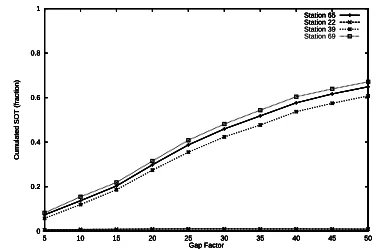
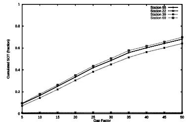
When varying the gap factor, the TTRT was chosen to be 20 msec and the request size was fixed at 14 bytes, thus yielding a load of approximately 20 % when all stations are in the ring (when the 9 bytes overhead of variable length telegrams are taken into account). For the case of independent errors we show the mean station outage time (MSOT) for every active station in Fig. 1 and the cumulated outage times (defined as the fraction of time that a station is not in the ring) are shown in Fig. 2. For the case of gilbert errors the MSOT is shown in Fig. 3 and the cumulated outage times are shown in Fig. 4. The following points are interesting:

3_{The assumption of a common channel simplifies the model; it does not necessarily hold on wireless links. The assumption, that the sender also}

[image:4.595.321.513.54.179.2]

(5)

0 0.2 0.4 0.6 0.8 1 1.2 1.4

5 10 15 20 25 30 35 40 45 50

MSOT (sec)

Gap Factor

Station 65

0 0.2 0.4 0.6 0.8 1 1.2 1.4

5 10 15 20 25 30 35 40 45 50

MSOT (sec)

Gap Factor

0 0.2 0.4 0.6 0.8 1 1.2 1.4

5 10 15 20 25 30 35 40 45 50

MSOT (sec)

Gap Factor

0 0.2 0.4 0.6 0.8 1 1.2 1.4

5 10 15 20 25 30 35 40 45 50

MSOT (sec)

Gap Factor

0 0.2 0.4 0.6 0.8 1 1.2 1.4

5 10 15 20 25 30 35 40 45 50

MSOT (sec)

Gap Factor

[image:5.595.99.283.53.190.2]

Fig. 3: MSOT vs. gap factor (Gilbert Errors)

0 0.2 0.4 0.6 0.8 1

5 10 15 20 25 30 35 40 45 50

Gap Factor

Station 65

0 0.2 0.4 0.6 0.8 1

5 10 15 20 25 30 35 40 45 50

Gap Factor

0 0.2 0.4 0.6 0.8 1

5 10 15 20 25 30 35 40 45 50

Gap Factor

0 0.2 0.4 0.6 0.8 1

5 10 15 20 25 30 35 40 45 50

Gap Factor

0 0.2 0.4 0.6 0.8 1

5 10 15 20 25 30 35 40 45 50

Gap Factor

[image:5.595.321.512.54.178.2]

Fig. 4: Cumulated SOT vs. gap factor (Gilbert Errors)

• For all stations except station 22 (lowest station address) the MSOT increases almost linearly with the gap factor. Even more, the slope is greater for higher station adresses. This can be explained as follows: when station 22 experiences two succes-sive hearback errors, it immediately removes it-self from the ring after the second token telegram. It sends no further data, especially no token. As described in section II, it then behaves as newly switched on, i.e. it has only an empty LAS. In this situation the token is lost and thus there is no activity on the medium. As a result, the time-out timer expires. But unfortunately, since 22 has the lowest station address, the timeout timer ex-pires first for station 22, which then claims the to-ken and thinks it is the only station in the ring, since there was no other transmission during the time between the removal of 22 and its timeout. Station 22 will send the next token to itself, all other stations feel themselves skipped and remove themselves from the ring. It will take then some time to re-include the stations. By the definition of the ring inclusion algorithm it is then clear that the mean time needed for re-including the station with higher addresses increases almost linearly with the gap factor.

• The results on the cumulated station outage time are dramatic: for gap factors of around 30 all ac-tive stations except station 22 are only 50 % of the time member of the ring. This gets worse for higher gap factors. Even for small gap factors these stations are for approximately 10 % of the time not member of the ring. This shows clearly that the used deterministic algorithm for station inclusion breaks down under a high bit error rate.

• Under the gilbert error model both the MSOT and the cumulated SOT are slightly higher for all sta-tions except station 22 than under the independent error model.

• Under the independent error model we have not observed any case where station 22 gets lost due

to being skipped by erroneous token telegrams of other stations. However, under the gilbert model this has happened a few number of times.

A first conclusion is that the gap factor should be pretty low in order to achieve at least a bad result for the frac-tion of time of being a ring member (as compared to the unacceptable results for higher gap factors). However, this has the drawback that more bandwidth is wasted for pinging stations. In practice it would also be a good idea to use consecutive station addresses in order to decrease the number of ping packets to unused station addresses. As next experiment we have varied the load, while keeping TTRT (20 msec) and gap factor (6) fixed. For the load we have chosen to keep the request size fixed (10 bytes) and to vary the interarrival time from 5 msec to 10 msec. For the case of independent errors the MSOTs are shown in Fig. 5 and the cumulative SOTs are shown in Fig. 6. As compared to the gap factor, here the MSOT and cumulated SOT are much less sen-sitive against varying load. Even more, for increasing load (smaller IAT values) the cumulated SOT decreases. This can be explained by the fact that with higher load there occur less token telegrams per fixed unit of time and thus less occasions to get lost from the ring. How-ever, even a cumulated outage time of approximately 4 % is not really acceptable for realtime applications.

IV.B Mean Delay

(6)

0 0.05 0.1 0.15 0.2

5 6 7 8 9 10

MSOT (sec) IAT (msec) Station 65 0 0.05 0.1 0.15 0.2

5 6 7 8 9 10

MSOT (sec) IAT (msec) Station 65 Station 22 0 0.05 0.1 0.15 0.2

5 6 7 8 9 10

MSOT (sec) IAT (msec) Station 65 Station 22 Station 39 0 0.05 0.1 0.15 0.2

5 6 7 8 9 10

MSOT (sec) IAT (msec) Station 65 Station 22 Station 39 Station 69 0 0.05 0.1 0.15 0.2

5 6 7 8 9 10

[image:6.595.96.284.53.330.2]

MSOT (sec) IAT (msec) Station 65 Station 22 Station 39 Station 69

Fig. 5: MSOT vs. IAT (Independent Errors)

0 0.05 0.1 0.15 0.2 0.25 0.3

5 6 7 8 9 10

IAT (msec) Station 65 0 0.05 0.1 0.15 0.2 0.25 0.3

5 6 7 8 9 10

IAT (msec) Station 65 Station 22 0 0.05 0.1 0.15 0.2 0.25 0.3

5 6 7 8 9 10

IAT (msec) Station 65 Station 22 Station 39 0 0.05 0.1 0.15 0.2 0.25 0.3

5 6 7 8 9 10

IAT (msec) Station 65 Station 22 Station 39 Station 69 0 0.05 0.1 0.15 0.2 0.25 0.3

5 6 7 8 9 10

IAT (msec)

[image:6.595.319.520.54.340.2]

Fig. 6: Cumulated SOT vs. IAT (Independent Errors)

0 0.002 0.004 0.006 0.008 0.01 0.012 0.014

5 6 7 8 9 10

Mean Delay (sec)

Interarrival Time (msec)

ideal,independent errors 0 0.002 0.004 0.006 0.008 0.01 0.012 0.014

5 6 7 8 9 10

Mean Delay (sec)

ideal,independent errors normal, independent errors

0 0.002 0.004 0.006 0.008 0.01 0.012 0.014

5 6 7 8 9 10

Mean Delay (sec)

ideal,independent errors normal, independent errors ideal, Gilbert errors

0 0.002 0.004 0.006 0.008 0.01 0.012 0.014

5 6 7 8 9 10

Mean Delay (sec)

ideal,independent errors normal, independent errors ideal, Gilbert errors normal, Gilbert errors

0 0.002 0.004 0.006 0.008 0.01 0.012 0.014

5 6 7 8 9 10

Mean Delay (sec)

Fig. 7: Comparison of Mean Delay with normal and idealized protocol under both error models with MBER = 0.001

0 0.0005 0.001 0.0015 0.002 0.0025 0.003 0.0035 0.004 0.0045 0.005

5 6 7 8 9 10

Mean Delay (sec)

ideal,independent errors 0 0.0005 0.001 0.0015 0.002 0.0025 0.003 0.0035 0.004 0.0045 0.005

5 6 7 8 9 10

Mean Delay (sec)

ideal,independent errors normal, independent errors

0 0.0005 0.001 0.0015 0.002 0.0025 0.003 0.0035 0.004 0.0045 0.005

5 6 7 8 9 10

Mean Delay (sec)

ideal,independent errors normal, independent errors ideal, Gilbert errors

0 0.0005 0.001 0.0015 0.002 0.0025 0.003 0.0035 0.004 0.0045 0.005

5 6 7 8 9 10

Mean Delay (sec)

0 0.0005 0.001 0.0015 0.002 0.0025 0.003 0.0035 0.004 0.0045 0.005

5 6 7 8 9 10

Mean Delay (sec)

Fig. 8: Comparison of Mean Delay with normal and idealized protocol under both error models with MBER = 0.0001

between issuing the request for transfer of data and the corresponding indication at the remote station (thus it in-cludes any retransmission before the first correct recep-tion). However, the delay is measured only for telegrams which are received correctly. For a proper interpretation of the curves we should note the fact that in our simula-tion every source does only generate requests when the corresponding station is currently member of the ring. It is reasonable to expect significantly higher mean delays, when this restriction is removed.

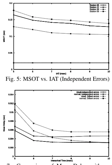
In Fig. 7 we show the results for a mean bit error rate of 0.001, both under the independent error model and under the gilbert model, when the interarrival time was varied. The results are worth some explanations:

• Under both error models the delay under the nor-mal protocol is significantly higher than under the ideal protocol, as is the delay variation and the maximum observed delay, both not shown here. This is mainly due to frames which are already in the stations queue, when the station is lost from the ring (we do not delete the requests when the station leaves the ring).

• It can be seen from Fig. 7 that, for the inde-pendent error model, for both the idealized pro-tocol and the normal propro-tocol the mean delay in-creases with increasing load (decreasing interar-rival time), however, for increasing load the graph of the normal protocol converges to the graph of

the ideal protocol. This can be explained by the observation that for higher loads there are less to-ken frames per fixed unit of time and thus less op-portunities for a station to get lost from the ring. The same observation holds for both protocols un-der the gilbert error model.

• For higher loads (interarrival time smaller than 7 msec) the ideal protocol under gilbert errors be-haves worse than the normal protocol under in-dependent errors. This can be explained by the bursty nature of channel errors: while the channel is in bad state, it is likely that a single frame ex-periences several consecutive retransmissions and thus stays longer in the queue. Due to the shorter interarrival times it is likely that new requests ar-rive meanwhile, which then queue up behind the first one and will be delayed longer.

[image:6.595.321.514.54.181.2] [image:6.595.324.520.203.339.2]

(7)

• The normal protocol under gilbert errors has al-ways approximately twice the mean delay as the ideal protocol under independent errors.

• The maximum observed delays and the delay vari-ance for the normal protocol under both error models is significantly higher than for the ideal-ized protocol. Thus the loss of control frames has a significant impact on delay variation.

In Fig. 8 we show the mean delays for a mean bit error rate of 0.0001, also under the independent error model and under the gilbert model with varying interar-rival times. The curves are almost identical. This is an indication that for this MBER the loss of control frames has no significant impact on the mean delay. The main reason is that it is very unlikely to loose two or three con-secutive token frames as compared to the MBER 0.001.

V DISCUSSION ANDCONCLUSIONS

In this paper we have gained some insight in the dy-namics and the behaviour of the PROFIBUS token pass-ing protocol over error prone links. We see the followpass-ing main results:

• The protocol is very sensitive to loss or corrup-tion of control frames, especially token frames. If some parameters are chosen bad (e.g. gap factors), the ring breaks completely down, at least under the relatively high mean bit error rate of 10−3_.

While significantly increased mean delays are a serious performance problem, the high percentage of cumulated station outage times is a catastrophe.

• For the unmodified protocol it seems to be the best to use small gap factors, subsequent station addresses and a high system load in order to de-crease station loss rate and cumulated station out-age times.

• The results are asymmetric in the sense that the station with the lowest address receives much bet-ter performance than all other stations. And even within the remaining stations higher station ad-dresses are a penalty. One can say that the lowest station determines the fate of the ring.

• If the MBER is a magnitude smaller (10−4_{) then}

things look better and station losses are rare.

• For delays and outage times the protocol has shown to be more sensitive against bursty error behaviour than for “smooth” independent errors.

In the technical report we have proposed several im-provements to the protocol and frame formats, two of them are evaluated by simulation, namely a new time-out computation method and a fast re-inclusion scheme. When combined they show a significant improvement in the cumulated station outage times. For improving the mean delays the timeout calculation method will suf-fice. However, the results are still not good for realtime-applications. For this reason we believe that for creating a wireless PROFIBUS the choice of the original protocol even with some modifications is not a good one.

REFERENCES

[1] E. O. Elliot. Estimates of error rates for codes on burst-noise channels. Bell Syst. Tech. J., 42:1977– 1997, September 1963.

[2] German Institute of Standardization (DIN). PROFIBUS Standard Part 1 and 2, 1991.

[3] E. N. Gilbert. Capacity of a burst-noise channel. Bell Syst. Tech. J., 39:1253–1265, September 1960.

[4] Hong ju Moon, Hong Seong Park, Sang Chul Ahn, and Wook Hyun Kwon. Performance Degradation of the IEEE 802.4 Token Bus Network in a Noisy Environment. Computer Communications, 21:547– 557, 1998.

[5] Mesquite Software, Inc., T. Braker Lane, Austin, Texas. CSIM18 Simulation Engine – Users Guide, 1997.

[6] K. Pahlavan and A.H. Levesque. Wireless Informa-tion Networks. J. Wiley and Sons, 1995.

[7] PROFIBUS Nutzerorganisation e.V., PROFIBUS Nutzerorganisation e.V., Haid-und-Neu-Str. 7. Im-plementation Guide to DIN 19245 Part 1, August 1994.

[8] H.S. Wang and N. Moayeri. Finite state markov channel - a useful model for radio communication channels. IEEE Transactions on Vehicular Technol-ogy, 44(1):163–171, February 1995.