MASTER THESIS
DEPLOYING SECURITY
FORCES TO INTERCEPT
THREATS
T.L.C. van der MIJDEN
ELECTRICAL ENGINEERING, MATHEMATICS AND COMPUTER SCIENCE APPLIED MATHEMATICS
INDUSTRIAL ENGINEERING AND OPERATIONS RESEARCH STOCHASTIC OPERATIONS RESEARCH
EXAMINATION COMMITTEE prof. dr. R.J. Boucherie dr. J.B. Timmer dr. G.J. Still dr. H. Monsuur
DOCUMENT NUMBER
Abstract
Management summary
Motivation
To protect valuable objects and critical infrastructure, security forces are often deployed to surveil and patrol assigned areas. The purpose of these forces is the interception of incoming threats before actual damage can be done. The question that arises in deploying security forces is how to deploy these forces optimally, i.e. where are these forces deployed most effectively?
Goals
This study’s purpose is to help answering this question. We assume that threats, e.g. terrorists, move through a network attempting to reach a certain destination. Security forces are deployed in this network to surveil network sections and intercept encountered threats. We take into account that security forces operate in a stochastic environment, one never knows when and where the next threat will emerge. We also allow for multiple active threats at the same time. The question we will answer is:
How to deploy security forces in the network in order to minimize the number of threats reaching their destination?
Furthermore, in direct application of our research, we consider counter-piracy operations in the Somali Basin. Pirates operating from Somalia, move to shipping routes to hijack passing merchant ships. To counter this piracy threat, naval ships are deployed in patrol areas to surveil maritime traffic and to intercept pirates. We investigate the optimal deployment of these naval ships.
Approach
To answer these questions, we study an interdiction game on a queueing network. An interdic-tion game describes how two adversaries compete over a value of a system. In our applicainterdic-tion, the two adversaries are the naval forces and the pirates and the value over which they compete is the number of successful pirate attacks. A queueing network allows us to incorporate the stochastic time environment and multiple threats.
Results
Preface
Around June 2010, I had my first appointment with the chair holder of the Stochastic Opera-tions Research (SOR) group, Prof. Dr. R.J. Boucherie, to discuss my graduation program at the University Twente. During this meeting we talked about my preference to apply opera-tions research within the military domain. Months before this first meeting, I had followed an academic minor in military sciences which rekindled my youth interest in military subjects. It was then, that I decided to explore the possibility to apply my math skills to problems arising from the military domain.
After being brought into contact with Dr. H. Monsuur of the Netherlands Defense Academy (NLDA), the research direction was established. It was no surprise that it would include both queueing theory, an expertise of the SOR group, and game theory, an expertise of the Opera-tions Research group at the NLDA.
The research started quite theoretical, which was fine for the beginning, but over time it brought down my motivation. New motivation came along with the opportunity to apply my research to counter-piracy operations in the Somali Basin. Commander P.J. van Maurik of the Royal Netherlands Navy was doing research on (counter-) piracy activity and could use my research to obtain some insight in optimal deployment of naval forces and its effect on piracy activity. Talking about naval ships, patrol areas and pirates instead of queues and customers was a welcome change.
I would like to thank everyone who has supported me during my graduation. In particular my thanks to my supervisors Richard Boucherie and Herman Monsuur, with the help of their knowledge, supervising skills and enthusiasm, I was able to bring forth this research. Also I would like to thank Peter van Maurik for giving me insight in the piracy problem in the Somali Basin and for all the interesting conversations we had. Thanks to all colleagues, fellow student, friends and family for all their support to me and my research.
Table of contents
Abstract i
Management Summary iii
Preface v
Table of contents vii
1 Introduction 1
1.1 Background . . . 1
1.2 Interdiction models . . . 3
1.2.1 Overview of interdiction models . . . 3
1.2.2 Literature on interdiction . . . 4
1.3 Goals . . . 6
1.4 Approach . . . 8
1.5 Report structure . . . 10
2 Basic model 11 2.1 Introduction . . . 11
2.2 Network description . . . 11
2.3 Stationary distribution . . . 13
2.3.1 A single isolated node . . . 13
2.3.2 The network . . . 14
2.4 Game description . . . 15
2.5 Link to a previous study . . . 17
3 Game analysis 19 3.1 Introduction . . . 19
3.2 Optimal mixed strategies . . . 19
3.2.1 No cycles . . . 19
3.2.2 Optimal mixed strategies . . . 22
3.3 Optimal pure strategy . . . 23
3.3.1 Convexity . . . 23
3.3.2 Optimal pure interdictor strategy . . . 25
4 Special cases 27 4.1 Introduction . . . 27
4.2 Parallel queues . . . 27
4.3 Tandem queues . . . 30
4.4 Model extensions . . . 32
4.4.1 Batch removals . . . 32
5 Application to anti-piracy operations 37
5.1 Introduction . . . 37
5.2 Problem description . . . 37
5.3 Anti-piracy model . . . 38
5.4 Queueing model . . . 40
5.5 Interception probability . . . 41
5.5.1 Approximation approach . . . 41
5.5.2 Maximum distance . . . 41
5.5.3 Interception probability . . . 42
5.6 The model . . . 45
5.7 The use of queues . . . 46
5.7.1 Motivation for queues . . . 46
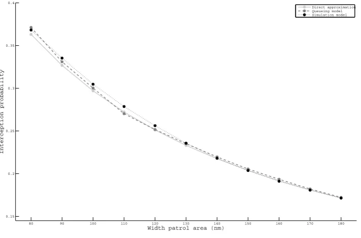
5.7.2 Verification . . . 46
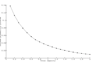
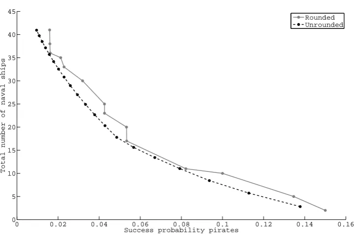
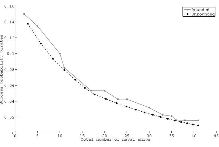
6 Results on anti-piracy deployment 49 6.1 Introduction . . . 49
6.2 Pirate’s success probability . . . 49
6.3 Use of UAVs . . . 54
7 Conclusions 57 7.1 Conclusions . . . 57
7.2 Discussion . . . 58
7.3 Further research . . . 58
References 59
1
Introduction
1.1
Background
Over the last decade, critical infrastructure protection has received considerable attention. Economy and society are more and more dependent on infrastructures such as energy, trans-port and telecommunications. This increases the need to identify and protect those infrastruc-ture elements that, if lost, would cause significant disruption of the (inter)national economy and society. The loss of infrastructure can be caused by random events (e.g. earthquakes) or intentional attacks (e.g. terrorist attacks). These causes constitute probabilistic respectively strategic risks to infrastructure. Protecting critical infrastructure against strategic risks is of great concern to homeland security, especially after the terrorist attacks of September 2001. Homeland security and protection is often a task of intercepting threats before any harm is done and is always faced with uncertainty, one will never know when the next threat will emerge. Here, threats may be interpreted as nuclear weapons being smuggled from country to country or pirates attempting to hijack merchant vessels. Another very topical interpretation is the threat of cyber-attacks, although much more interpretations are possible.
To intercept threats security forces may rely on intelligence and respond whenever a new threat emerges. However security forces may also be deployed, actively surveilling areas and searching for threats. The latter case is often applied when threats occur regularly, e.g. pirate attacks in the Somali Basin. Although threats may arrive regularly, the time of appearance is always uncertain. This is inconvenient, because in order to intercept a threat one has to be at the same place at the same time. On the other hand, security forces themselves cannot be predictable in their search patterns and schedules, since that would surely be exploited by those imposing the threats.
In the context of piracy, the Somali Basin is a current stage for such a problem. In 2011 there were 160 pirate attacks reported in de Somali Basin and even more attacks were at-tributed to pirates operating from Somalia. Over the last years, this number of pirate attacks has increased vastly. Therefore, several coalitions and countries have sent naval ships to the area to surveil maritime activity and intercept pirates. Due to the expanse of the area, a single naval ship has to cover a great area and cannot surveil the whole assigned patrol area at any time and timing is crucial in the interception of pirates.
When deploying security forces with the task of surveilling and patrolling certain areas, the purpose is to minimize the number of threats that become actual attacks. The question that arises is; how to deploy the available security forces in the most effective manner, i.e. to min-imize the number of threats not being intercepted. This question is the main focus of this research.
that most homeland security issues are strategic in nature. To help decision-making in strate-gic environments, game theory provides a way. Much research has been done in the area of
game-theoretic risk analysis applied to homeland security and defense (see e.g. Bier and Azaiez
(2009)). An important class of game-theoretic models in the field of homeland security and defense are interdiction models. Brown et al. (2006) apply such an interdiction (or
attacker-defender) model to assess infrastructure vulnerability to intentional attacks. These interdiction
1.2
Interdiction models
1.2.1 Overview of interdiction models
An interdiction model describes an infrastructure system and its value, including how the ac-tions of two adversaries influence this value. The two adversaries, often called the interdictor and the operator, have opposite goals; while the operator’s goal is to maximize the value of the system, the interdictor attempts to minimize this value. Interpretation of the value may be very different depending on the actual system being modeled. For example the value may mean financial profit, production capacity or probability of non-detection. Interdiction models have a wide range of applications including hospital infection control (Assimakopoulus (1987)), electric power grid protection (Salmeron (2004)), ballistic missile defense (Brown et al. (2005)) and interdiction of a nuclear-weapons project (Brown et al. (2009)). Most interdiction models
areStackelberg games; the interdictor and operator perform their actions sequentially.
Further-more, since the interdictor and operator have opposite goals, these games arezero-sum games. To solve these Stackelberg games, the models are regularly formulated as bi-level (integer) pro-grams, see for example Brown et al. (2006). An important class of interdiction models focuses on systems that can be described by a network consisting of arcs and nodes. This leads to the concept of network interdiction models.
Network interdiction models are optimization models, in which the interdictor performs
in-terdiction actions on a network in order to minimize the maximum value the operator can obtain from the network. The network consists of nodes connected by arcs. In literature two models have received considerable attention. The first is the maximum flow network
interdic-tion model. In this model the value to the operator is determined by the amount of flow he
1.2.2 Literature on interdiction
Since in literature considerable attention is given to the maximum flow and shortest path inter-diction models, we give an overview of the literature following this subdivision. In themaximum
flow network interdiction model the operator maximizes the flow of some commodity from a
source node through the network to an end node, while the interdictor attempts to minimize this flow by interdicting (e.g. removing) network components. One of the first to explore this field was Wollmer (1964), who was concerned with removing a fixed number of arcs in a network in order to minimize the maximum flow through the network. Corley and Chang (1974) also considered this model, but their interdiction actions consisted of removing a fixed number of nodes from the network. The maximum flow network interdiction model was gener-alized by Wood (1993), who considered interdiction costs for removing arcs. The interdictor in this case is constrained by an interdiction budget. Wood also showed the NP-hardness of the problem and developed an integer programming model. Phillips (1993) considered the case in which the decrease in arc capacity is linear in the interdiction efforts put in that arc. Other research was done by Lim and Smith (2007) and Royset and Wood (2007), who considered respectively models with multiple commodity flows and models in which the interdictor mini-mizes both the maximum flow and the interdiction costs. Stochastic variants of the maximum flow network interdiction model were studied by Cormican et al. (1998) and Janjarassuk and Linderoth (2008). In those models arc capacities and interdiction successes can be stochas-tic. Recent studies of Altner et al. (2010) and Zenklusen (2010) deal with the development of the methods of finding an optimal solution for the maximum flow network interdiction problem.
Theshortest path network interdiction model considers an operator whose objective is to
de-ception, effectively creating asymmetric information. Cappanera and Scaparra (2011) develop a multi-level optimization model to solve the shortest path network interdiction problem in which network components can be hardened, making them invulnerable to interdiction.
In the models described above, the interdictor and the network user move sequentially. First the interdictor changes the network, after which the operator optimizes his value using the altered network. However, there are some studies in which the interdictor and the operator choose their actions simultaneously. Washburn and Wood (1995) consider a shortest path network interdic-tion model, in which arc lengths are interpreted as detecinterdic-tion probabilities. In their model an evader attempts to travel across a network undetected, while an interdictor sets up an inspec-tion point. The evader chooses a path to travel and the interdictor chooses an arc to inspect, both making their decision without knowing the decision of their adversary. If the inspected arc is part of the chosen path, then the evader is detected with a certain probability. This problem establishes a normal zero-sum game, where the players choose a randomized strategy. Another study, done by Washburn and Ewing (2011), models a traffic network under threat by Improved Explosive Devices (IEDs). In this model a number of traffic units move over road segments per unit time. An interdictor places IEDs with a certain rate on these road segments, aiming to inflict maximum damage to the traffic. Simultaneously, the network user deploys IED clearance units, resulting in the removal of IEDs without damaging any traffic. The problem constitutes a game which is played indefinitely in time. Alpern et al. (2011) present a patrolling game. In this game, an attacker chooses to perform an attack on a certain node in a network. This attack will take some time periods, in which the attacker may be detected by a patroller. This patroller chooses a patrol schedule through the network, this schedule describes where the patroller is located in each time period. If the location of the patroller at some time period co-incides with the location of the attacker, the attacker is intercepted and the patroller wins. This study provides insight to help schedule patrols through museums and other vulnerable facilities.
1.3
Goals
Although the literature on network interdiction models is quite extensive and useful in the area of homeland security, there are some aspects that have not received much attention and yet may be relevant factors.
First of all, literature lacks time-dependent interdiction models. In the studies on interdic-tion, the focus is on static, time-independent models. The maximum flow interdiction models consider static flows and in the shortest path interdiction models, the operator is not actually moving along the path in time. In addition literature describes, with some exceptions, interdic-tion models in which timing of interdicinterdic-tion acinterdic-tions is not relevant. However, one can imagine situations in which units are actually moving through the network in time and where inter-diction actions can only be executed in certain time windows. For example, the interception of a terrorist can only take place after its detection and before it reaches its destination and causes some harm (e.g. see Wein and Atkinson (2007)). Also, one can only interdict a task of a weapons manufacturing project when it is not yet finished. Besides, like in the case of a terrorist interception, one often cannot use the same interdiction resource (e.g. a police car) for multiple interdiction efforts at the same time. Although timing is crucial in intercepting threats before they become actual attacks, few studies incorporated a time element in their research.
The second aspect arises from the evader-detection models like in Washburn and Wood (1995). In these models only single evaders are considered. Multiple evaders or threats are not con-sidered. Yet it is not unlikely that multiple threats are active at the same time and while intercepting a first threat, a second threat may pass unchecked. So the notion of multiple threats is one of quite importance in interdiction models.
The application of the theory that will be developed in this study deals with the deployment of security forces to intercept threats. Deployed forces surveil and patrol assigned areas and in-tercept encountered threats. We will take into account that these forces operate in a stochastic time environment; threats emerge at random points in time and search patterns and schedules have some degree of unpredictability. Moreover since patrolling forces are often deployed to counter threats which appear frequently, we allow for multiple active threats at the same time. Our concern will be to deploy the available security forces in the most effective manner.
In direct application of the theory we discuss counter-piracy operations. To counter piracy in the Somali Basin, maritime patrol areas are established and naval ships are allocated to these areas to intercept pirates moving to shipping routes. Our objective will be to allocate the available naval ships in order to minimize the number of successful pirate attacks by intercept-ing them durintercept-ing their transit to their areas of operation.
the operator sends through the network. We will considerdynamic network flows, i.e. flows of which units are actually moving through the network in time. Moreover we assume that each single flow unit is vulnerable to interception while moving through the network. The model relates to both the maximum flow and shortest path network interdiction. Each single flow unit can be seen as a single threat attempting to reach its destination undetected, yet together the threats constitutes a flow, which is to be maximized by the operator.
An interdictor and an operator compete over these network flows. The interdictor aims to minimize the value the operator can obtain from the dynamic flow network, while the operator tries to maximize this value. We will mainly be concerned with models in which the value will be determined by the number of flow units reaching their destination, i.e. the throughput. However, also other values may be considered, such as the expected travel time from source to destination for a single flow unit (provided the flow unit reaches its destination), or the probability that at least a certain fraction of the flow reaches its destination. Furthermore the operator may route different types of flow units through the network, each type with its own value.
The interdiction strategy will consist of the allocation of security agents to the network. Agents will intercept flow units (threats) if they are at the same location at the same time. Several allocation strategies may be considered. Each agent may be allocated to a specified location or may patrol several locations. Also agents can be stationed at a base location and move from this base to other network locations. Furthermore, detection and interception can be separated by introducing detection sensors to the network, like in Yates et al. (2011). Other cases may consider agents that act dependent on available information.
The main research question in the context of the counter-piracy application is:
• How to allocate available naval ships to patrol areas in order to minimize the number of
successful pirate attacks?
In the development of the theory we generalize this to:
• How to deploy available interception resources in a dynamic flow network in order to
1.4
Approach
To model dynamic flow networks and the actors on these networks, we will combine two sepa-rate areas of research; game theory and queueing theory. Where game theory provides a way to model the interaction between the interdictor and the operator, queueing theory can be used to model the dynamic flows and time-dependent interdictions in a stochatic environment. In queueing models, the movement of a flow unit, usually called a customer, is actually modelled in time; the unit arrives at a certain time at the queue, there it has to wait and/or receives service for some time and then moves on, possibly to another queue. Since a queueing model describes precisely where a flow unit is located in the system at a given time, it is also possible to intercept this unit at a certain time and location. Moreover queueing theory gives us tools to model interaction between customers and/or agents.
Although there are some studies that incorporate queueing theory in their analysis, the use of queueing theory in the area of interdiction models remains virtually unexplored. Atkinson and Wein (2008) and Yates et al. (2011) use respectively a spatial queueing model and a hy-percube queueing model to analyze the performance of interception units chasing vehicles that pose a potential threat. Further, in the research of Washburn and Ewing (2011) an infinite-server queue is used to model the number of IEDs located on a road segment. But apart from these studies, queueing models and interdiction models are rarely combined.
In our research we use queueing theory to model and analyze the time-dependent behavior in our interdiction models. We replace the usual network of nodes and arcs in network inter-diction models by a network of interconnected queues. In these networks of queues, customers (flow units) move through the network via several queues. At the queues the customers have to stay for some time, possibly depending on the presence of other customers. These customers are called positive or regular, because upon arrival at a queue they increase the number of cus-tomers at this queue. We use the notion of negative cuscus-tomers, introduced by Gelenbe (1991), to model the agents who intercept the flow units. Upon arrival at a queue, negative customers remove a regular customer, if present, from that queue. Removed customers are interpreted as intercepted customers and do not add to the throughput of the network. Now the problem is described as follows. The operator has to route the regular customers through the network in order to maximize the throughput. The interdictor on the other hand decides on the arrival rates and routing of the negative customers, while aiming to minimize the throughput.
The main research question can be reformulated as
• What are optimal strategies for the interdictor and operator in a queueing network in
order to maximize, respectively minimize the throughput of the network?
To answer this question, first the following subquestion are answered:
• Do there exist optimal strategies for the interdictor and the operator?
• If optimal strategies exist,are we able to find them in general and/or specific cases?
Several distinctions in the models can be made with regard to the type of the queue and the characteristics of the negative customers.
Type of the queues
Our main focus is on the single server queues, but one may also consider infinite server queues. In networks of single server queues, the time a customer spends at a queue is dependent on the number of other customers present at that queue, this in contrast to a network of infinite server queues. In these networks the time spend at a queue by a customer is independent of other (regular) customers.
Customer removal policies
Upon arrival of a negative customer at a queue, several removal policies can be considered. The negative customers may remove only one customer (e.g the one being served), a subset of the present customers or it may remove all customers it finds present at that queue. Furthermore, in case only one customer is removed, the removed customer may have been any of the present customers or a specific one, e.g. the customer that arrived first at that queue.
Negative customer allocation
1.5
Report structure
2
Basic model
2.1
Introduction
To address the allocation problem of security forces in a network to intercept threats effectively, a model needs to be developed. This section descibes the formation of an interdiction game on a queueing network. The part concerning the interdiction game incorporates the aspect of an intelligent opponent, while the part involving queueing theory incorporates the stochastic time environment and the notion of multiple threats. In the first section the network is described, where each node of the network represents a queue. Thereafter some basic analysis is given concerning the stationary distribution of the network and the probability of intercepting a threat. In section 2.4 the game is descibed, with action sets and payoff function. The last section relates the described model to a model already studied in literature.
2.2
Network description
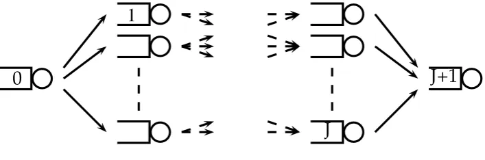
Let G be a network with source node 0, sink node J + 1 and a set of intermediate nodes
I ={1, . . . , J}, see figure 1. The whole set of nodes is denoted by V, V ={0,1, . . . , J, J + 1}. The set of links in the network is denoted by E, node j is connected to node k if (j, k) ∈ E. The forward star F S(j) of node j is the set of all nodes k for which (j, k)∈ E, i.e. F S(j) =
{k|(j, k)∈E}. Likewise, the backward starBS(j) of nodej is the set of all nodes k for which (k, j) ∈ E, i.e. BS(j) = {k|(k, j) ∈ E}. A path l is a finite sequence of nodes (l1, . . . , lm(l)) such thatli ∈V fori= 1, . . . , m(l) and (li, li+1)∈Efori= 1, . . . , m(l)−1, wherem(l) denotes the length of path l. We denote by L the set of all possible paths from node 0 to node J+ 1. A simple path is a path in which no node is visited twice, i.e. a path without cycles. The set of all simple paths is denoted by ¯L.
We assume that in G there are no links entering node 0, i.e. BS(0) = ∅, and there are no
links leaving node J + 1, i.e. F S(J + 1) = ∅. Furthermore we assume that there is at least one path from node 0 to node J+ 1, but there is no link between node 0 and node J + 1, i.e. (0, J + 1)∈/ E.
0
1
J
[image:21.595.124.478.614.731.2]J+1
Each node in the network G represents a queue where regular (or positive) customers arrive and are served by a single server according to a FIFO service discipline. These customers arrive
from the outside of the network at node 0 according to a Poisson process with rate γ. The
total arrival rate of regular customers at queue j is denoted by λ+j. The service time at node
j is exponentially distributed with mean 1/µj. After service completion at node j, a regular
customer is routed to node k with probability r(j, k). Regular customers leave the network
after finishing service at node J + 1. We refer to R as the transition matrix with elements
r(j, k). Since customers can only leave the network at nodeJ + 1 we have
J+1
X
k=0
r(j, k) = 1, for j = 0, . . . , J. (1)
Furthermore, customers cannot be routed over links that do not exists, so
r(j, k) = 0, ∀(j, k)∈/ E.
In addition to regular customers also negative customers arrive at queues j ∈ I. The concept of negative customers was first introduced by Gelenbe et al. (1991). Upon arrival of a negative customer a regular customer, if present, is removed from the network. If a negative customer arrives at an empty queue, the negative customer simply disappears. Negative customers do not receive service and are not routed through the network. Negative customers arrive at queue
2.3
Stationary distribution
2.3.1 A single isolated node
The state of the network process can be described by the number of regular customers present at each node. Let nj be the number of regular customers present at node j, the state is given
byn = (n0, n1, . . . , nJ+1). Our aim is to find the stationary distribution of the process, i.e. to find the probability that in equilibrium the network is in state n. This probability is denoted by π(n). In order to determine the stationary distribution, we first consider a single node in isolation.
Consider node j in isolation and let πj(nj) denote the stationary probability that there are
nj customers present at node j in equilibrium. The process satisfies the following balance
equations.
λ+jπj(0) = (µj +λ−j)πj(1), (2)
(λ+j +µj +λ−j )πj(nj) = λ+j πj(nj −1) + (µj+λ−j )πj(nj + 1), nj ≥1. (3)
Equation (2) and (3) arise from balancing the probability flows in equilibrium. The solution to these equations is given by
πj(nj) = (1−ρj)ρ nj
j , nj ≥0, (4)
where
ρj =
λ+j µj+λ−j
(5)
and provided thatρj <1. Note that this node with negative customers has the same dynamics
as an ordinary M/M/1 queue with arrival rate λ+j and service rate µj +λ−j . The arrival of
negative customers with Poisson rate λ−j has the same effect on the stationary distribution as increasing the service rate of the node with λ−j .
Let qj be the probability that a regular customer leaves node j due to a service completion.
This probability equals the departure rate due to service completion at node j divided by the total departure rate at nodej. In equilibrium the total departure rate equals the total arrival rate. So we have,
qj =
ρjµj
λ+j , (6)
= µj
µj +λ−j
. (7)
Likewise, we have the probability that a customer is removed by a negative customers at node
j,
1−qj =
λ−j µj+λ−j
One can obtain these probabilities also via some other reasoning. First assume that a negative customer will remove the regular customer in service. (This assumption may be dropped, but it helps to get some idea about the dynamics of the queue.) Both the interarrival time of a negative customer and the service time of a regular customer are exponentially distributed. The probability that a customer completes its service equals the probability when entering the service, the service time is smaller than the time until the next arrival of a negative customer. This probability equals the probability that an exponentially distributed variable with mean 1/µj is smaller than an exponentially distributed variable with mean 1/λ−j , this is precisely
given by equation (7).
2.3.2 The network
In the network the arrival rates of regular customers are given by the traffic equations,
λ+j =
J
X
k=0
ρkµkr(k, j), j = 1, . . . , J + 1, (9)
λ+0 = γ. (10)
Here, ρk is given by equation (4). Let ej be a vector of lengthJ+ 2 with the (j+ 1)th element
equal to 1 and zeros elsewhere. Like in the case of a single node we can establish the balance equations which are satisfied by π(n).
π(n)
J+1
X
j=0
λ+j + (µj +λ−j)1[nj >0] = J+1
X
j=0
π(n−ej)λ+j1[nj >0] +π(n+ej)(µj+λ−j ), ∀n,
(11) where 1[x] = 1 if x is true and 0 otherwise. Now, by quasi-reversiblity of M/M/1 queues, the stationary distribution of a network of M/M/1 queues is given by the product of the stationary distribution of each node in isolation. Since the dynamics of the nodes in our network are the same as an ordinary M/M/1 queue, we derive that the stationary distribution of the network is given by
π(n) =
J+1
Y
j=0
πj(nj), ∀n ≥0. (12)
with πj(nj) given by equation (4).
Remark. For a more extensive discussion of queues with negative customers and networks
2.4
Game description
In the described network, an operator and an interdictor compete over the throughput of the
network; the departure rate of regular customers at node J + 1. The operator aims to
maxi-mize this throughput by choosing an appropriate routing matrix R. The interdictor attempts
to minimize the throughput by deciding on the arrival rates of the negative customers at the nodes. The resulting game is a zero-sum game, i.e. what the operator gains on throughput is lost by the interdictor.
The action set from which the operator can choose its action is given by
Aoperator =
( R J+1 X k=0
r(j, k) = 1 for j = 0, . . . , J, r(j, k)≥0, ∀(j, k)∈E, r(j, k) = 0 ∀(j, k)∈/ E
)
.
(13) The action set from which the interdictor can choose is given by
Ainterdictor =
( λ− J+1 X j=0
λ−j ≤Λ−, λ−j ≥0, ∀j, λ−0 =λ−J+1 = 0
)
. (14)
The interdictor is constrainted in its action by a total arrival rate Λ− of negative customers to the network. The payoff of this game is given by the departure rate of regular customers at nodeJ+ 1. Since there are no arrivals of negative customers at node J+ 1, the departure rate of this node equals its arrival rate. We have, given R and λ−, a payoff of
v(R, λ−) =λ+J+1. (15) As λ+J+1 is determined by R and λ− via equation (5), (9) and (10), this payoff is defined im-plicitly.
A strategy for a player is a probability distribution over the set of actions of that player. A strategy for the operator is a measureF defined on the setAoperator such that F(Aoperator) = 1.
Similary, a strategy for the interdictor is a measure G defined on the set Ainterdictor such that
G(Ainterdictor) = 1. A pure strategy for either player is a measure that gives measure 1 to a
single element of the action set of that player. So, a pure strategy for the operator will be a measureF such thatF(R) = 1, this means that with probability 1 the operator chooses action
R. A strategy which is not pure, is called a mixed strategy. The expected payoff is defined as
E(F, G) =
Z
Aoperator×Ainterdictor
v(R, λ−)d(F ×G), (16) =
Z
Aoperator
Z
Ainterdictor
v(R, λ−)dG(λ−)dF(R),
=
Z
Ainterdictor
Z
Aoperator
Define the following two numbers
vI = sup
F
inf
G E(F, G), (17)
vII = inf
G supF E(F, G). (18)
The first question is whether or notvI =vII. If vI =vII then the game is said to have a value.
If furthermore also sup inf and inf sup can be replaced by max min and min max respectively, then there exist optimal strategies.
Section 3 will answer these questions, but first recall the payoff function. This payoff func-tion, given by equation (15), equals the rate at which regular customers arrive at node J+ 1. Hence, these customers have left every node they had visited due to service completion,
oth-erwise they would have been removed from the network by a negative customer. Let l be a
path from node 0 to node J+ 1, then the probability that a customer, moving along this path, arrives at nodeJ + 1 and leaves the network due to service completion equals
m(l)−1
Y
i=1
qli, (19)
whereqjis given by equation (7). From the transition probabilities we can derive the probability
that a pathl will be travelled by a customers, this probability equals
m(l)−1
Y
i=1
r(li, li+1). (20) By conditioning on the path travelled by a customers, the probability that an arbitrary customer arrives at nodeJ + 1 equals
X
l∈L m(l)−1
Y
i=1
r(li, li+1)qli. (21)
Multiplying by the total arrival rate at node 0, we obtain the rate at which customers arrive at node J+ 1, and thus
v(R, λ−) =γX
l∈L m(l)−1
Y
i=1
r(li, li+1)qli. (22)
Note that the set L of all possible paths from node 0 to node J + 1 has an infinite number of elements; a path may include an arbitrary number of cycles. In section 3.2 we prove that we can restrict the summation in (22) to all simple path from node 0 to nodeJ+ 1, i.e. replace L
2.5
Link to a previous study
As special case of the game descibed in the previous section may be interpreted as a general-ization of the game described in Washburn and Wood (1995). Suppose that instead of deciding on the arrival rates of the negative customers, the interdictor can only decide on which nodes negative customers will arrive. The action of the interdictor is descibed by the vectorx= (xj),
wherexj = 1 if the interdictor chooses nodej and 0 otherwise. The action set of the interdictor
is given by
¯
Ainterdictor =
( x X
j∈I
xj ≤M, xj ∈ {0,1}, ∀j ∈I
)
. (23) HereM denotes the capacity constraint of the interdictor. Suppose furthermore that if xj = 1
that negative customers will arrive at node j according to a Poisson process with given rate
λ−j . Then the payoff function is given by
¯
v(R, x) = γX
l∈L m(l)−1
Y
i=1
r(li, li+1)
µli
µli+xliλ
−
li
, (24)
= γX
l∈L m(l)−1
Y
i=1
r(li, li+1) 1−
λ−l
i
µli +λ
−
li
xli
!
. (25)
If xj = 1 a customer is removed at node j by a negative customer with probability
λ−j µj+λ−j
.
Each regular customer is routed independently of each other regular customer, furthermore also the removal probabilities of a regular customer at the nodes are independent of other regular customers. As a consequence this game is equivalent to the game, played repeatedly, in
which only one regular customer is routed from node 0 to node J+ 1. This is exactly a game
3
Game analysis
3.1
Introduction
In the previous section, a new interdiction game is described. In this section we are concerned with the existence of optimal strategies in this game. First we will look for optimal mixed strategies. In doing so, we deal with routing strategies of the operator which result in positive customers being routed in cycles. After establishing a result concerning optimal mixed strate-gies, we consider optimal pure strategies. To prove existence of an optimal pure strategy for the interdictor, convexity of the payoff function has to be analysed.
3.2
Optimal mixed strategies
3.2.1 No cycles
A routing strategyR∗ is optimal for a given λ− if
R∗ = arg max
R v(R, λ
−
). (26)
Furthermore we say thatR contains a cycle if there exists a node for which the probability that it will be visited more than once by the same customer is strict positive.
Theorem 1. There exists an optimal R for every λ− such that R does not contain any
cycle.
Before we prove the theorem, we first prove a slightly easier lemma.
Lemma 1. If λ−j > 0 then node j cannot be contained in a cycle in an optimal routing
matrix R∗.
Proof of Lemma 1. Define ηj as the marginal benefit to the operator in the throughput
of routing an additional customer through node j. Under the optimal routing matrix R∗, ηj
satisfies the following relations
η0 = max
k∈F S(0)ηk, (27)
ηj =
µj
µj +λ−j
max
k∈F S(j)ηk, ∀j ∈I, (28)
ηJ+1 = 1. (29) If a customer is routed through node j, then with probability λ
−
j
µj+λ−j
this customer is removed
by a negative customer and the operator gains nothing. With probability µj
µj+λ−j the customer
is routed to a next nodek∗ and the benefit equalsηk∗. Since underR∗ the operator maximizes
Moreover, the marginal benefit of an additional customer is only strictly positive if the customer eventually reaches nodeJ+ 1. Since λ−j ≥0, it follows that
0< µj µj +λ−j
≤1, ∀j ∈I (30)
and thus we deduce from (28) that whenever a customer is routed under R∗ from node j to
nodek the following must hold
ηj ≤ηk. (31)
Letc= (c1, . . . , cm, c1) be a cycle contained in R∗. From (31) follows
ηc1 ≤ηc2 ≤. . .≤ηcm ≤ηc1, (32)
which yields,
ηc1 =ηc2 =. . .=ηcm =ηc1. (33)
In order for equation (33) to hold, we must have that λ−ci = 0 for every ci. Equivalently, if
λ−j >0 node j cannot be contained in a cycle. Hence, we have proven the lemma.
Proof of Theorem 1. Let λ− be given and suppose that the optimal routing matrix R∗
contains a cycle. Define λ+j,k as the flow of regular customers moving along link (j, k), we have
λ+j,k =λ+j µj µj+λ−j
r(j, k). (34) As before let c = (c1, . . . , cm, c1) be a cycle contained in R∗. From Lemma 1 follows that for every node ci contained in a cycle we haveλ−ci = 0 and thus
λ+ci,ci+1 = λ+cir∗(ci, ci+1), i= 1, . . . , m(c)−1, (35)
λ+cm,c1 = λ+cmr∗(cm, c1). (36)
We will now construct a new routing matrix R∗∗ from R∗ which does not contain the cycle c
and is also optimal. Let eλ+j and eλ+j,k denote respectively the total flow through nodej and the
flow along link (j, k) under the new routing matrix R∗∗. We construct R∗∗ as follows. First define the flow of regular customers along the whole cyclec by
ζc= min i λ
+
ci,ci+1. (37)
Next, substract a flow of ζc from every link (j, k) contained in the cycle c and maintain the
same flow for every other link.
e
λ+ci,ci+1 = λ+ci,ci+1 −ζc, i= 1, . . . , m(c)−1, (38)
e
Consequently the total flow through every node ci in c is reduced by ζc. The total flow of all
other nodes remains equal.
e
λ+ci =λ+ci −ζc, i= 1, . . . , m. (40)
Note that all flows into a node and all flows out of a node are still balanced. Now, define R∗∗
by the following equation
r∗∗(j, k) =
e
λ+j,k
e
λ+j if eλ
+
j 6= 0,
r∗(j, k) if eλ+j = 0.
(41)
It is easy to see thatR∗∗∈Aoperator: If nodej is not contained in the cyclecor satisfiesλe+j = 0,
there is no change in the transition probabilities from these nodes, i.e. r∗∗(j, k) = r∗(j, k). Furthermore for each nodeci in the cycle cfor which eλ+c
i >0, we have
X
k
r∗∗(ci, k) =
X
k
e
λ+c
i,k e λ+ ci , (42) = P kλ +
ci,k−ζc
λ+
ci−ζc
, (43)
= 1. (44)
MoreoverR∗∗still satisfies the conditionsr∗∗(j, k)≥0∀(j, k)∈E andr∗∗(j, k) = 0∀(j, k)∈/ E. So, R∗∗ is a feasible action for the operator. Also the cycle cis not contained in R∗∗, since for
i∗ being the argument of the minimization in (37) we have,
e
λ+c
i∗,ci+1 =λ
+
ci∗,ci+1−ζc= 0 (45)
and hence
r∗∗(ci∗, ci∗+1) = 0. (46)
3.2.2 Optimal mixed strategies
Theorem 1 shows that for every action of the interdictor, the operator has an optimal action which does not result in customers moving along cycles. As a consequence, there exists a optimal strategy for the operator in which the probability that a customers moves along a cycle is zero. Hence, we can limit summation in the payoff function, as given in equation (22), to the finite set of all simple paths. The payoff function becomes
v(R, λ−) = X
l∈L¯ m(l)−1
Y
i=1
r(li, li+1)qli. (47)
This payoff function is continuous, because the set ¯Lis finite. The following theorem is due to Glicksberg (1952).
Theorem 2. In a two person zero-sum game, if the action sets of both players are compact and
the payoff function is continuous, then the game has a value and optimal mixed strategies exist.
Clearly the setsAoperatorandAinterdictor are compact and since the payoff function is continuous,
3.3
Optimal pure strategy
3.3.1 Convexity
Now we have established a result that guarantees the existence of optimal mixed strategies, we like to investigate the existence of optimal pure strategies. However, first we are concerned with the convexity of the payoff function, for convexity will be sufficient condition for pure strategies. Recall that the payoff function is given by
v(R, λ−) =X
l∈L¯
m(l)−1
Y
i=1
r(li, li+1)
µli
µli +λ
−
li
. (48)
Lemma 2. Let the parametersµi, i= 1, . . . , n be given and strictly positive. The function
f(x) =
n
Y
i=1
µi
µi+xi
(49)
is strictly convex on the set {x|xi ≥0, i= 1, . . . , n}.
Proof of lemma 2. A function is strictly convex if and only if its Hessian matrix is
pos-itive definite. So we prove that the Hessian of f(x) is positive definite to establish the result. The Hessian ∇2f(x) is given by
[∇2f(x)]
i,j =
∂2f(x)
∂xi∂xj
, i, j = 1, . . . , n, (50) where
∂2f(x)
∂x2
i
= 2
(µi+xi)2
f(x), (51)
∂2f(x)
∂xi∂xj
= 1
(µi+xi)(µj +xj)
f(x), i6=j. (52) We know that ∇2f(x) is positive definite if all leading principal minors are positive. Denote byMm the mth leading principal minor, then
Mm =
X
σ∈Sm
sgn(σ)
m
Y
i=1
[∇2f(x)]i,σi. (53)
where the summation is taken over all permutations of the set {1, . . . , m}. The key is to note that in each term a product is taken overmelements. Each of thesem elements are taken from different rows and columns. Due to the structure of the second partial derivatives off(x), we have that each product of elements will be equal to
cσ
(f(x))m (gm(x))2
wherecσ is a constant depending on the permutation σ and
gm(x) = m
Y
i=1
µi+xi. (55)
As a consequence
Mm =
(f(x))m (gm(x))2
X
σ∈Sm
sgn(σ)cσ. (56)
It turns out that
X
σ∈Sm
sgn(σ)cσ (57)
equals the determinant of a m×m matrix with diagonal elements equal to 2 and 1 elsewhere.
We denote this matrix by H, furthermore let v be a vector of lenght m with all elements equal to 1. With I the identity matrix, we have
H =I+vvT. (58) Now it follows from the equality
I 0
vT 1
I+vvT v
0 1
I 0
−vT 1
=
I −v
0 1 +vTv
(59)
that
det(H) = 1 +vTv =m+ 1. (60)
It follows that the leading principal minors are given by the following equation
Mm =
(m+ 1) (f(x))m (gm(x))2
, m= 1, . . . , n. (61) Since µi > 0 and xi ≥ 0 for all i, each Mm > 0. We thus conclude that ∇2f(x) is positive
3.3.2 Optimal pure interdictor strategy
With this preparatory result established, we can state the following theorem.
Theorem 3. The interdictor has an unique optimal pure strategy.
Proof of theorem 3. Rewrite the payoff function v(R, λ−) as
v(R, λ−) =X
l∈L¯ m(l)−1
Y
i=1
r(li, li+1) m(l)−1
Y
i=1
µli
µli+λ
−
li
. (62)
We recognize thatv(R, λ−) is a linear combination of functions fl(λ−), with
fl(λ−) = m(l)−1
Y
i=1
µli
µli+λli
, l∈L.¯ (63)
As a result of lemma 2, these functions are strictly convex and hencev(R, λ−) is strictly convex inλ− forλ− ∈
λ−λ−i ≥0 . Therefore, since the action sets of both players are compact, we
4
Special cases
4.1
Introduction
The previous sections were concerned with a general game model on a queueing network. Section 2 gave a description of the queueing network and the game that is played upon the network. After which, section 3 gave results on the existence of optimal strategies. This section considers special cases of the described game. On a network of parallel queues and a network of tandem queues, we provide optimal strategies for the operator and the interdictor. Sections 4.2 and 4.3 give these results. Furthermore section 4.4 extends the game of the previous sections to a game in which negative customers may remove more than one positive customer from a queue.
4.2
Parallel queues
Consider the network in which the nodesj ∈I are in parallel with each other, i.e. r(j, J+1) = 1
∀j ∈ I. In this network regular customers can move along paths of the form l = (0, j, J + 1) with j ∈I. The payoff function in now defined by
v(R, λ−) =γX
j∈I
r(0, j) µj
µj +λ−j
. (64)
This function is convex inλ−and linear inR, and thus also concave inR. FurthermoreAoperator
and Ainterdictor are compact and convex sets. It can be proven that in this case optimal pure
strategies exists (Fan (1953)). In other words
v = max
R minλ− v(R, λ
−
) = min
λ− maxR v(R, λ
−
). (65)
The operator has only to decide on the values of r(0, j) ∀j ∈I, thus every action R is a linear combination of the actions Rj in which r(0, j) = 1, j ∈I. Due to the linearity of v(R, λ−) in
R and the fact that each R is a linear combination of the actions Rj, we can find the optimal
λ− by solving the following minimization problem. min
λ− w (66)
subject to
γ µj µj+λ−j
≤w, ∀j ∈I. (67)
The constant w is interpreted as the maximum payoff the operator can obtain, which is
min-imized by the interdictor. Furthermore, due to the linearity in R we only need to make sure
that v(R, λ−)≤ w for R =Rj ∀j ∈ I. Now since v(R, λ−) is continuous in λ−, we have that
for an optimalλ−∗
γ µj µj+λ−∗j
Rewriting yields
λ−∗j = γ−v
v µj, ∀j ∈I. (69)
Using
X
j∈I
λ−∗j = Λ− (70) gives us,
Λ−=X
j∈I
γ−v
v µj (71)
or
γ−v v =
Λ−
P
j∈Iµj
. (72)
Finally we obtain the optimal λ−∗ by combining equations (69) and (72),
λ−∗j = Pµj
k∈Iµk
Λ−, ∀j ∈I. (73)
The value of the game is given by
v =
P
j∈Iµj
P
j∈Iµj+ Λ−
γ. (74)
So, given the capacity constraint Λ−, the network of parallel nodes with service rates µj is
equivalent, in terms of the throughput, to a system of one node with service rate P
j∈Iµj.
Furthermore, the value and the optimalλ−∗ are independent of the action of the operator, i.e. given that the interdictor chooses actionλ−∗, the operator’s action choiceR does not influence the payoff of the game. However, for every R there is a unique optimal λ−, since v(R, λ−) is strictly convex in λ−. Hence, there is a unique R∗ which should be played by the operator in order to guarantee at least a payoff equal to the value of the game. ForR∗ must hold
γX
j∈I
r∗(0, j) µj
µj+λ−j
≥v =
P
j∈Iµj
P
j∈Iµj + Λ−
γ. (75)
Suppose we chooseR such that
r(0, j) = Pµj
k∈Iµk
, ∀j ∈I. (76) Forλ− ∈Ainterdictor the payoff is given by
v(R, λ−) = P γ
k∈Iµk
X
j∈I
µ2j µj+λ−j
. (77)
strategy for the operator. When giving it some thougths, one can obtain a quite intuitive interpretation for the form of the optimal strategy. The payoff depends on the probability qj
that a customer is not removed by a negative customer. This probability, given in equation (7), depends on the time a customer spend in service; the smaller the service time, the greater the probability of service completion. In this network of parallel nodes, the operator can choose those nodes which yields the smallest service times. Since all service times are stochastic, the operator should choose a node with probability equal to the probability that this node has the smallest service time. All service times are exponentially distributed, hence the probability that a node j has the smallest service time is given by
µj
P
k∈Iµk
, (78)
4.3
Tandem queues
Consider the network in which the nodesj ∈I are in tandem, i.e. r(i, i+1) = 1 fori= 0, . . . , J.
In this network regular customers can only move along one path from node 0 to node J + 1,
visiting each node in the network. The payoff function for this network is given by
v(λ−) =γY
j∈I
µj
µj+λ−j
. (79)
Since the operator has no choice in how to route the regular customers through the network, the interdictor action is found by just minimizing v(λ−) subject to the constraint
X
j∈I
λ−j = Λ−. (80)
The lagrangian of the problem is given by
ν(λ−, ψ) =γY
j∈I
µj
µj+λ−j
+ψ X
j∈I
λ−j −Λ−
!
. (81) Taking partial derivatives yields
∂ν ∂λ−j =
−1
µj +λ−j
v(λ−) +ψ ∀j ∈I, (82)
∂ν ∂ψ =
X
j∈I
λ−j −Λ−. (83) Equating the partial derivatives to zero results in
1
µj+λ−j
= ψ
v(λ−), ∀j ∈I. (84) Rewriting gives
λ−j = v(λ
−)−ψµ
j
ψ , ∀j ∈I. (85)
Summing equation (85) overj yields
Λ− = X
j∈I
v(λ−)
ψ −µj
, (86)
= v(λ −)
ψ J−
X
j∈I
µj. (87)
Rewriting gives
v(λ−)
ψ =
Λ−+P
j∈Iµj
Combining equation (85) and (88) gives
λ−j = Λ
−+P
k∈Iµk
J −µj, ∀j ∈I. (89)
These are the values which the interdictor has to choose to minimizev(λ−), provided that
0≤λ−j ∀j ∈I. (90)
Suppose that we have for somek, λ−k <0. We can find an optimal feasible solution by setting
λ−k = 0, and minimizev(λ−) over all λ−j, j 6=k. We can repeat this procedure until conditions (90) are met.
Equation (89) can be rewritten as
λ−j −
P
k∈Iλ
−
k
J =−
µj−
P
k∈Iµk
J
, ∀j ∈I. (91) This equation shows that the difference between the arrival rate of negative customers at a specific node and its mean over all nodes equals the difference between the service rate at that node and the mean service rate over all nodes, up to a minus sign.
If equation (89) is rewritten as
λ−j +µj =
P
k∈Iλ
−
k +µk
J , ∀j ∈I, (92)
we see that the rates at which regular customers leave the queues, given that the queues are not empty, are equal. This implies that when a queue has a smaller service rate, the rate at which negative customers arrive in the optimal strategy will be higher. This is explained as follows. In queues with smaller service rates, regular customers stay longer in service and thus are vulnerable to interception during a longer time period. Since the operator has no choice in routing the regular customers, the interdictor can put his resources there where these customers are most vulnerable: queues with low service rates.
The value of this game played on a network of tandem queues is given by
v =γY
j∈I
J µj
Λ−+P
k∈Iµk
4.4
Model extensions
4.4.1 Batch removals
Instead of considering special networks, also some extensions with regard to the queues can be made. The first extension is to assume that arriving negative customers may remove a batch of positive customers. The queueing network with batch removals is described and analyzed in Gelenbe (1993). Following the same method as Gelenbe (1993), we describe the interdiction game on a queueing network with batch removals.
A single queue
Before analyzing the whole network, consider a single server queue with exponentially dis-tributed service time with mean 1/µ. Positive customers arrive at this queue according to a Poisson process with rateλ+. In addition to these customers, also negative customers arrive at the queue according to a Poisson process with rate λ−. Upon arrival of a negative customer,
a batch of B positive customers are removed from the queue according to some probability
distribution; P(B = s) = ps, ps ≥ 0 ∀s,
P
sps = 1. Since all interarrival times and service
times are exponentially distributed, we do not have to know which customers are removed to determine the stationary distribution of the number of present customers, but we assume that regular customers are removed based on a ‘first in first out’-procedure. For this queue we have the following balance equations,
(λ++λ−)π(0) = µπ(1) +λ−
∞
X
n=0
π(n) ∞
X
s=n
ps, (94)
(λ++µ+λ−)π(n) = λ+π(n−1) +µπ(n+ 1) + ∞
X
s=0
π(n+s)ps, n >0. (95)
Suppose π(n) =cρn, then from (94) and (95) we obtain
λ++λ− = µρ+λ−
∞ X n=0 ρn ∞ X
s=n
ps, (96)
λ++µ+λ− = λ+1
ρ +µρ+λ
− ∞
X
s=0
ρsps. (97)
Define
f(x) = 1−
P∞
s=0x
sp s
1−x . (98)
Both (96) and (97) are equivalent to
ρ= λ +
µ+λ−f(ρ). (99) If (99) has a solution such thatρ <1, then the stationary distribtion is given by
If p1 = 1, f(ρ) = 1 and we have the queueing model described in section 2.2. If p∞ = 1, we have a queue with disasters (see Chao (1995))), i.e. negative customers which empty the whole queue upon arrival. In this case we have f(ρ) = 1/(1−ρ).
The function f can be rewritten as follows.
f(x) = 1−
P∞
s=0x
sp s
1−x , (101)
=
P∞
s=0ps−
P∞
s=0x
sp s
1−x , (102)
=
P∞
s=0(1−x
s)p s
1−x , (103)
=
P∞
s=0
Ps−1
t=0 (1−x)x
tp s
1−x , (104)
=
P∞
t=0
P∞
s=t+1(1−x)x
tp s
1−x , (105)
= ∞ X t=0 ∞ X
s=t+1
xtps. (106)
If we tag an arbitrary customer at a queue, the probability that there are t customers in front of this tagged customer equals ρt. From this we can see that f(ρ) equals the probability that an arriving disaster removes an arbitrary tagged customer.
A network of queues
In a network of J single server queues with batch removals, let µj be the service rate of queue
j and let λ−j denotes the arrival rate of negative customers at queue j. Upon arrival at queue
j a negative customer removes s customers with probability pj,s. Define
fj(x) =
1−P∞
s=0xspj,s
1−x . (107)
The traffic equations are given by
λ+j = X
k
ρkµkr(k, j), (108)
λ+0 = γ. (109)
where
ρj =
λ+j µj+λ−j fj(ρj)
. (110)
If (108) has a non-negative solution {λ+j } such that
then the stationary distribution of the network is given by
π(n) =Y
j
(1−ρj)ρ nj
j . (112)
The probability that a customer leaves queue j unintercepted equals
ρjµj
λ+j =
µj
µj +λ−jfj(ρj)
, (113)
which depends on both λ−j and λ+j . This might become a problem in analyzing the game, as
λ+j depends on the routing matrix R. Game description
The game on the network of queues with batch removals is only changed with respect to the payoff function. The action sets of both the operator and the interdiction remain the same and are given by (13) and (14). The payoff is also still given by the throughput of the system, however the explicite expression of the payoff function in (22) is changed, for the probability that a customer leaves the queue due to a service completion is changed. The payoff function is now given by
v(R, λ−) = γX
l∈L m(l)−1
Y
i=1
r(li, li+1)
µli
µli+λ
−
lifli(ρli)
. (114)
Sinceρj is a solution of equation (110) and we cannot write ρj explicitly in terms ofλ−,R and
µj, we cannot give an explicite expression of the payoff function in terms of the chosen actions
of both players. As yet, this is an obstacle in our path to analyze this game any further.
4.4.2 Other queueing models
Routing negative customers
Another extension would be to route not only the positive customers through the network, but also the negative customers. In literature the routing of negative customers is often taken into account in studying queues with negative customers, see e.g. Gelenbe (1991). However in these studies the routing of negative customers relies on the presence of positive customers at the queues. Negative customers disappear from the network if they arrive at an empty queue. The routing of negative customers is taken into account by a probability that a positive customer leaving a queue is routed as a negative customer to a next queue.
empty queues are not studied in literature. In particular we cannot give an expression of the stationary distribution of such a network and thus we cannot analyse an interdiction game played on such network.
Infinite server queues
5
Application to anti-piracy operations
5.1
Introduction
In the previous chapters we developed an interdiction model which takes time-dependency into account as well as multiple interdictor and operator units. In this section we apply the model to an actual problem which has become more and more pressing over the last couple of years; piracy. First the problem is described, after which the developed model is slightly adjusted and applied to the problem. The last section presents the results.
5.2
Problem description
The threat to international shipping formed by pirates operating from Somalia has increased over the last couple of years, despite the military presence of various countries and coalitions. Piracy in the form of hijacking merchant ships began in 2003 in the Gulf of Aden and expanded in 2005 along the whole coast of Somalia. However, due to the increased military activity and the abandonment of the shipping routes near Somalia, pirates moved their operating areas increasingly farther away from the Somali coastline. Nowadays pirates operate as far as 1000 nautical miles (nm) from the Somali coastline.
Although the probability that a merchant ship is hijacked, is very small, the effects of piracy on the international trade and economy are large. The estimated cost of piracy is around eight billion dollars per year. Although this cost is relatively low compared to the turnover of ship-ping companies the influence is major, for the profit margins are small.
5.3
Anti-piracy model
The problem is modelled as a zero-sum game as descibed in section 2.4. The pirates and naval forces compete over the number of succesfull pirate operations. The pirates may choose their operating area(s) in their attempt to increase the number of succesfull hijacks. Naval forces have established patrol areas and decide on the number of ships allocated to each area in order to minimize the number of succesfull hijacks.
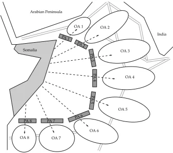
Figure 2 gives an schematic representation of the Somali region. Pirates operating from Soma-lia have multiple operating areas (OA) in which they may attempt to hijack passing merchant vessels. With each operating area i, a parameter gi is associated. The parameter gi indicates
the pirate’s probability of a succesful operation, given that the pirate reaches operating area
i. This parameter depends on the traffic density in the area, the distance from shore and also military presence in the operating area. (This military presence in the operating areas in not taken into account beyond the parameters gi.)
To reach an operation area, pirates have to transit through a maritime patrol area (PA). During their transit through a patrol area, pirates are vulnerable to interception. The patrol
Arabian Peninsula
Somalia
India
PA 1 PA 2
PA 3
PA
4
PA
5
PA 6
PA 7 PA 8
OA 1
OA 6 OA 2
OA 3
OA 4
OA 5
[image:48.595.120.477.430.745.2]OA 7 OA 8
areas are modelled as queues with arrivals of positive and negative customers, see section 2.2 and 2.3. The arrival of a pirate at a patrol area and its transit is represented by an arrival of a postive customer to a queue and its service at this queue. The removal of a positive customer due to an arrival of a negative customer represents the interception of a pirate by a naval ship.
5.4
Queueing model
The key in the first part of the model is to derive optimal interception probabilities for each patrol area, by determining the optimal arrival rates of naval ships. LetJ denote the number of patrol areas. The interception probabilities of pirates, i.e. the removal probabilities of positive customers, depend solely on the arrival rate of naval ship and the transit time through the area and not on the arrival rate of the pirates themself (see section 2.3). Let 1/µj be the
deterministic service time of the pirates at queuej, then the interception probability at patrol area j is given by the probability that the interarrival time of the naval ship is less than 1/µj.
Let λ−j denote the arrival rate of the negative customers at queue j, then the interception probability at patrol area j is given by
P(Interception at j) = 1−e−λ−j/µj, j = 1, . . . , J. (115)
The payoff is given by the number of pirates per unit time that succesfully complete their operation. These are pirates that are not intercepted by naval ships and when arrived in their operating area perform a succesfull hijack. Let r(0, j) be the probability that a pirate will attempt to move through patrol area j. Then, given R = (r(0, j)) and λ− = λ−j
, the payoff function is given by
v(R, λ−) = γ
J
X
j=1
r(0, j)e−λ−j/µjg
j. (116)
Since all patrol areas are in parallel, the optimal solution for this problem can be found in a similar way as in section 4.2. A strategy λ− is optimal if for all j it holds that,
v =γe−λ−j/µjg
j. (117)
Using the capacity contraint of the interdictor, i.e.
J
X
j=1
λ−j = Λ−, (118)
we can solve equation (117) forλ−. Rewrite equation (117) as
λ−j =µjloggj +µjlog
γ
v. (119)
Summing overj, using the capacity contraint and rearranging the terms yields logγ
v =
Λ−j −P
kµkloggk
P
kµk
. (120)
From both equation (119) and (120) we deduce that the optimal strategy λ−∗ is given by
λ−∗j = Pµj
kµk
Λ−+X
k
µklog
gj
gk
!
. (121)