Nonlinear wave groups in deep water

NONLINEAR WAVE

~GROUPS

IN

DEEP WATER

by

P. J. Bryant

No.

13

August

1978

1.

Nonlinear wave groups in deep water

BY P.J. Bryant

Nonlinear wave groups in deep water consist of wave modes for

which nonlinear interactions and dispersion are in balance. The

evolution equations for the wave modes are derived, and properties

of nonlinear wave groups are found from these equations. It is

shown that the nonlinear wave groups are linearly unstable to

side-band modulations in the sense that the linearised perturbation

theory, in providing a good fit over the initial time interval,

predicts that the growth of the modulations is exponential. Instead

the perturbed wave group is shown to return cyclically to a state·

close to its initial state. The cyclic recurrence is demonstrated

analytically for the simpler wave groups and numerically otherwise.

The interactions between nonlinear wave groups of the same and of

2.

1. Introduction

A wave group in deep water·contairitn9 a narrow waveband of wave

modes propagates, to a first approximation, with the group velocity of

the central wave mode in the waveband. The linear theory predicts that

the wave modes will disperse slowly causing the group to disintegrate

as it propagates. The nonlinear theory shows that weak nonlinear

inter-actions between the wave modes can balance the weak dispersion so that

the envelope of the wave group keeps a permanent shape.

The method of analysis used here is based on the representation of

a wavetrain c:>f periodically spaced wave groups by a Fourier series, the

series consisting of linear wave modes with amplitudes which vary slowly

with time. Evolution equations for the Fourier amplitudes are calculated

in terms of the nearly resonant tertiary interactions between the wave

·modes. This approach has its origins in the investigation by Benney and

Newell [1] of the mechanics of the propagation of nonlinear wave

envelopes. Their method was applied to deep water wave groups by Cohen,

Watson and West [2], and is expanded further in the present investigation.

The alternative approach to nonlinear wave groups is by the use of

model equations [ 3, 4, 5; 6], principally the cubic Schrodinger equation.

A derivation of this equation for a narrow waveband wavetrain is to be

found in (7], §17.7, where it is shown also that such a wavetrain in

deep water is unstable in the sense that small modulations to the

wave-train grow exponentially in time. Yuen and Lake [8] found good agreement

between experiments on deep water narrow waveband nonlinear wave groups

and the corresponding numerical solutions of the cubic Schrodinger

equ~tion, and the initial modulational instability has been demonstrated

experimentally by Lake, Yuen, Rungaldier, and Ferguson

[91.

The latter

experiments were continued to longer times to show that the modulations

3.

atate close to its initial state (in agreement with a previous numerical

calculation by Roskes [10)). These properties are all confirmed by the

present investigation.

The inverse scattering method may be applied to the cubic

Schrodinger equation ([.71, §17 .9), when it is found that the nonlinear

wave groups (soliton envelopes) retain their structure after interactions

with one another. This property has been verified experimentally by

Yuen and Lake

[8].

The method fails for nonlinear wave groups of the

same central wavenumber propagating with the same velocity, so

calculations are made here of the interactions between nonlinear wave

groups of the same and of almost the same central waven\wiDers.

2. Evolution equations

The water surface displacement has the form of periodically spaced

wave groups, the spacing of the groups being 2TIL .. The central wave mode

of each group has wavelength 2TI1, so that ko

=

L/1 is the nondimensional

wavenumber at the centre of the waveband, all wavenumbers being

non-dimensional multiples of 1/L. The space coordinates are x in the

direction of wave propagation, and y vertically upwards from the mean

free surface, both being nondimensional multiples of L The time t is

.a nondimensional multiple of

(1/g)~.

The maximum trough to crest height

of the·wave group envelope is 2a, and E =a/lis the principal small

parameter. The water surface displacement n(x,t) is a·nondimensional

multiple of a, and the velocity potential ~(x,y,t) is a nondimensional

multiple of

a(gl)~.

The governing equations may then.be written

~

+

~

...

0

4> + 0 aa y + - m ,

n

+

«<>t

+

en«~> t

+

&:ic($2 + «!>~> + l:ir2

<rtzcfl )

Y

X

Y

YY

t

+ c2nn t«<> = O(c3) on y = o. x -x

The Fourier series expansions for

n

and «!> are

n ...

1:! I: ~ (t) exp i (kx/ko - !1\kt) + i<

k

4>

=

~ I: Ck ( t) exp (ky /ko) exp i (kx/ko - wkt) +

k

4.

(2.lb)

(2.lc)

(2.1d)

(2. 2a)

(2.2b)

where

*

denotes complex conjugate and the Fourier amplitudes ~, ck are

slow functions of t. The linear theory yields

~

=

-i(ko/k)l:i

~

+ 0(£)

~

"" (k/ko) 1:! •

( 2. 3a)

(2.3b)

The quadratic theory describes sum interactions between wave modes

of wavenumbers ~, .k-~ and difference interactions between wave modes of

wavenumbers ~~ k+~ to produce wave modes of wavenumber k. The resulting

contributions to the Fourier amplitude ~ are estimated by

and

respectively. None of the quadratic interactions is near resonance for

the dispersion relation (2.3b), so these contributions to~ are only

0(£) compared with ~ itself •

. The tertiary interactions may be separated into two kinds,· those

·.that are significant because they are near resonance, and those whose

contribution to ~ is not significant because they are not near resonance.

When the three interacting wave modes as well as the resulting wave mode

all have wavenumbers in the ~,eighbourhood of ko, their contribution to

5.

ul

+

Ill - IIJ·0 • - ltlk

m k+9,-m •

+

(k

+

!1, - m - ko) 2 - ( Jl. - ko) ? - (k - ko) 2) •

The above contribution to ~ is 0(1), of the same magnitude as ~ itseu,

when all wavenumbers k in the narrow waveband centred on k0 are such that

(2.4)

The amplitude paramter £ is mucp smaller than 1, so for this relation

to be satisfied,

ko

must be much greater than 1. For this reason, the·

present investigation is restricted to narrow wavebands centred on

wave-numbers ko

>

1 for which significant tertiary interactions occur.between

the wave modes present.

None of the remaining tertiary interactions ;Lies near resonance, so

none contributes significantly to ~· One such tertiary interaction is

the sum interaction between three of the wave modes present to produce

an 0(£2) wave mode with a wavenumber near 3k_{0 •} A less obvious tertiary

interaction is that between a quadraticaliy generated 0(£) wave mode and

an 0(1) linear wave mode to produce an 0{£2) wave mode, as for example

when the 0(£) correction to equation (2.3a) is multiplied with an 0(1)

amplitude .A in the expansion of the third term of equation (2.lc).

The derivation of the evolution equations is now st'raightforward.

The Fourier series (2~2a,b) are substituted into equations (2.lc,d),

the quadratic terms are neglected completely, and the only tertiary

terms retained arethose for quartets of wavenumbers k, !1,, m, k+Jl.-m in

the neighbourhood of ko, with the Fourier amplitudes

c,

A in the tertiary

terms related by equation (2.3a). Equations (2.lc,d) become (with

6.

k+9..-l

L (

R.w$1, + mol + pw ) A~ A 1\

m=l m p m P

X

exp - i (W +

w

-IJ)n -Ill.. ) t. = 0,

· m p x, k (2.5a)

2 00 _k+fL-1

E: \' \'

+ ::::-2 l. l. { (W11

-w

-w ) (-$1,wn +roW +pW )

8k() fL=l m=l Jlv m P . N m p

+ 2 (mw W + iWnW + pW0hl ) }A! A A exp- i (W + W - W0 - W. ) t = 0 ~ ( 2. 5b)

m p· N :m "" p "" m p m p "' .k

The amplitude

Ck

is eliminated now between these two equations, and the

symmetry between m and k+t-m(=p) used to simplify the interaction

coefficient, when the evolution equation for ~

\_s

found to be

where

-k{ (k+t)w w

R = m P

k$1,m .

+

(3t+m)wtwm

+

(3t+p)u.I.II,Wp -

2tw

9

~}

ak!

(wm +wp- wt

+~)

(2.6a)

(2.6b)

Each w in this formula is given by equation (2.3b). Since the wavenumbers

in, p, !L, k all lie in a narrow waveband near

ko,

the interaction coeffic:ient

~tm may be approximated by

R _

.!. (

₁ + 9 (k - ko )

ktm

=

2 · 8k₀ + 11 ( fL - ko ) ) +

o(k -k

0 )

2

Bko · ko • (2.7)

An envelope function F(x,t) is introduced by rewriting the Fourier

series (2.2a) as

=

~F(x,t) expi(x-t) + = 1)

·where

ko+kl ( . )

F(x,t)=

L

~(t)expik~

0

kox-(~-l)t

If

the interaction coefficient 1\ll.m is approximatacl by-~- and the

dilperoion relation (2.3b) is approximated by

,

..

l+k-k1)

2k0

. 2

(k- ko)

skJ

it is found from equation (2.6a) that F(x,t) satisfies the cubic

Schrodinger equation

7.

(2.8a)

(2.8b)

{2.9)

The first two terms of this equation describe propagation of F with the

gro~p velocity~~

and the last two terms, which from relation (2.4) are

of comparable small magnitude, describe the weak dispersion and the weak

nonlinearity respectively. Most previous investigations have discussed

nonlinear wave groups as solutions of the cubic Schrodinger equation

(2.9), but the present investigation concentrates on those properties

of nonlinear wave groups which are obtained from the evolution equati.ons

. (2.6).

· 3 • Wave groups

The wave group solutions of the evolution equations are now

calculated. The two parameters describing .the shape of a wave group

are the.nondimensional amplitude £and the nondimensional central wav~

number kg. Relation (2.4) for the width of the waveband indicates that

the number of wavelengths in each group is proportional to 1/£, and

hence that the ra~io of the length of the group to the distance between

groups is proportional to 1/ (ko £) • The propagation velocity of the

8.

as e:: tends to zero, this velocity being

t

in the nondimensional multiples used. The simplest method of ensuring that in the wave group calculations

the centre·of the waveband remains in the neighbmirhood of k0 is by

1

setting the propagation velocity equal to

2

for all values of c. The

peak of the wavenumber spectrum then changes continuously in position as

e: is increased, but remains in the neighbourhood of k0 •

The Fourier series describing nonlinear wave groups pt·opagating

with velocity

t~

containing waves of central wavenumber 1 and central

frequency 1, is

expi(x-t)exp -ia.e:2t + .,., (3.la)

where from equation (2.2a),

~(t) ak exp 1 ( . wk - 1 - k-ko 2

2ko - a.e: ) t , (3.lb)

The amplitudes ~ are constants, the first three terms of the phase of

~are together O(e:2t}. (from equations (2.4.) and (2.8)), and the unknown

. part of the phase is written a.e:2t to give ~ the slow time dependence

indicated by the evolution equations (2.6).

The equations determining ~ (ko - kt ~ k

<:

ko + k1 ) and a. are therefore

ko - kt e;;; k ~ ko + kt , (3.2a)

together with the geometric constraint imposed by the definition of

e:,

namely

(3.2b)

For any given ko and e:, theS'P.J 2k1 + 2 equations are solved for the

9.

Newton-Raphson technique. The bandwidth 2kt is increased step by step

until no further change occurs in all variables to the precision

required (usually l0-4).

The nonlinear wave group for ko

=

40, £

=

1/40, is sketched 1n

figure 1. The amplitudes~ are plotted in figure l(a), and a= 0.251. One wavelength of the corresponding water surface displacement

n

is

s~etched in figure l(b). The amplitudes ~·and water surface

displace-ment

n

for ko

=

40, E

=

1/10 are sketched in figure 2 for comparison,

and a

=

0.262 in this example. The solitary nonlinear wave group

solutions of the cubic SchrOdinger equation (2.9) may be written

for which

and

sech TI (k-ko )

2 fiko E

(3.3a)

(3.3b)

The.re is good agreement between the solutions in figures l and 2, and

equations (3.3), apart from a slight asymmetry present in the sketched

solutions for ~· It is noted in this respect that the leading terms

in the omitted part of the contributions of the interaction coefficient

(2.7) and the Taylor series (2.8) to the cubic Schrodinger equation are

[image:10.595.77.551.48.642.2]

tel,

4 ~ ·Linear inetahi l i

.!:X

Benjamin and Feir [11] showed that a progressive wavetrain in

deep water is unstable, in the sense that a sideband modulation grows

exponentially in time during the initial time interval in which the

amplitude of the modulation remains small •. Lake et al [9] found more

recently that over longer times the amplitude of the modulation increases

and decreases, with the modulated wavetrain returning cyclically close

to its initial state.

Benjamin and Feir analysed a wavetrain of fundamental wavenumber k

and frequencyw interacting with sideband wave modes of wavenumbers

k(l

±

K) and frequencies W(l

±

6) where K' and

o

are sn1all fractions. The

essence of the instability mechanism is that a significant interaction

occurs within the qu~rtet with wavenumbers k, k, k ( 1 + K) , k ( 1 - K) and

frequencies w,

w,

W(l +

o),

W(l-

o)

respectively, causing the two

side-band wave modes to grow at the expense of the fundamental wave mode.

In a nonlinear wave group, significant interactions occur within all

quartets with wavenumbers k, 1, m, k+t-m in the neighbourhood of ko.

If one such wave mode is perturbed or is.itself a small amplitude

modulation, it can be expected therefore that the significant interaction

with the other three wave modes will cause this perturbation or modulation

to grow exponentially. This property is now confirmed. It can be

expected also thatover longer times the perturbed nonlinear wave group

will return cyclically close to its initial state, and this property is

confirmed in the following two sections.

The Fourier series for a given nonlinear wave group is that stated

in equation (3.1a). In order to investigate the stability and evolution

of a perturbed nonlinear wave group, it is preferable to use a Fourier

series for the water surfac~ displacement which has the same form as

11.

1 . k- ko 1 2

11

= 2

~ Bk (t) exp 1. ko (x -

2t)

exp i (x- t) exp- ia€: t +

*,

(4.la)

where

k - ko _ 2

1\(t)

=

Bk(t) expi(~- 1

-2ko cxe: )t.

The evolution equation for Bk, from equation (2.6a), is

where B '

k

=

ie:

2

I: E R 11 B! B Bk ·11 ,

51, m kx.m IV m +JV-m

( 1 k - ko ) /"' 2

Pk

=

~ ~

-

-

2ko ~

(4 .lb) .

( 4. 2)

(4. 3)

approximatelyr for wavenumbers k near k0 •

The wavenumber of the perturbing wave mode is denoted by K, where

ko - kt ~ K ~ ko + k1 , and its complex amplitude is aK + BK if K coincides

A

with one of the (integer) wavenumbers present, or is B otherwise.

K

Linearisation with respect to

B

in the tertiary interaction terms of

equation (4.2) indicates that the perturbed wave modes present have.

wave numbers 'K + n, n = 0, ± 1, ± 2, •.. , and 2ko - K + n, n

=

0, ± 1, ± 2, . . . . The evolution equations, linearised with respect to the perturbations

"

B, are

B'

ie:2 P .

B

=

ie:2 ( E I: R a a

B

K+n K+n K+n tm K+n,t,m t m K+n+t-m

+

I: E R a a

a*

) ,

t m K+n,ko+t- K,m m ko+n+t-m k0+2-K

(4.4a)

s'

_2ko-K+n ie:2 P _{2ko -K+n 2ko -K+n}

8

=

ie:2 (E E R a a

B

51, m 2ko -K+n, Q., m .IJ. m 2ko "':' K+n+ Q.-m

+

E E R a a

a*

) .

t m 2ko-K+n,K+t-k0 ,m m k0+n+t-m K+t-k0 (4.4b)

The system of first order linear differential equations with constant

coefficients consisting of equations (4.4a) with the complex conjugates

1?..

amplitudes B A , n

=

0 , ± 1 , ± 2 , ... , and B A* ,

K+n · · 2k.₀ -K+n n=O, :tl, ±2, . . . .

The method of solution of this system of differential equations for

any given values of

e::,

k.o and K has been described previously

( [ 12], §4), and is as follows. The system of differential equations

is reduced to a system of filgebraic equations by seeking normal mode

A

solutions for which each amplitude B has the same slow time dependence

exp(i~E2_t).

The system is then solved for the range of wavenumbers

within the waveband ko - kt

<

k

<

ko + kt • · The width 2k1 of the waveband

is increased step by step until the common eigenvalues A of consecutive

sets of equations agree to within an arbitrary numerical precision.

The system is stable if all eigenvalues

A

are real, unstable if any

pair of eigenvalues are complex conjugates. The solutions for the

A '

amplitudes B resulting from any given initial conditions may be

calculated from the eigenvectors of the set of algebraic equations.

Examples have been calculated for a range of values of£, k0 , and

K, and in every example there was at least one pair of eigenvalues ~

that were complex conjugates. The conclusion is that nonlinear wave

groups are unstable to small pertubations of the wave modes composing

them, and are unstable to small amplitude sideband modulations at other

wavenumbers near ko. The amplitudes. of the unstable modes were found

to decrease asK moved away from ko, which is to be expected because

the interactions. within the quartets of wavenumbers then move further

from resonance.

The eigenvector corresponding to each eigenvalue·~ is dominated

for almost every

A

by ~ unique complex amplitude

Bk,

enabling

A

to be

identified with a unique wavenumber k. This identification leads to

an interpretation for ~ in terms of a coefficient Qk for those

wave-numbers k outside the immediate neighbourhood of k0 • When all terms

u.

side of this equation, this side may be rewritten

8'

-

ic20

B .·,

K+n 'K+n K+n

where

(4. 5)

The normal mode ablutions of equation (4.4a) are those solutions for

It was found in all the examples.calculated that

A

tended towards the corresponding value of Qk ask tended away from k0 •

The values of A and Qk are listed in the following table for the first

example described below, for which ko

=

K

=

100.

k 95 96 97 98 99 100 101 102 103 104 105

Qk 3.243 2.076 1.174 0.535 0.153 0.025 0.146 0.515 1.125 1.975 3.061

A 3.245 2.079 .1.180 0.550 0.250 0. 530 1.131 1. 978' 3. 063

Table 1.

-4

The complex pair of eigenvalues (1.25 ± 2.63i) XlO has a pair of

complex eigenvectors which contribute significantly to all three central

amplitudes §99,

Bt

00 , §toi. Ask tends away from ko and A tends towards

pk, the contribution of the normal mode solution to

n,

from equation

(4.la), is dominated by

tsk exp i {kx - (wk

+

t:2 E

a~)

t}

+

*

5I,

(4.6)

where bk is a constant, and

~51,51,

is approximated by -

~

(equation 2. 7).

It follows that ·PElrturbations or modulations withwavenumbers outside

the immediate neighbou~hoqd of ko propagate almost as linear waves,

with only an.0(£2) correction to their linear frequency of similar form

to the amplitude correction for the frequency of Stokes waves in deep

.water. This is consistent with the property that nonlinear interactions

are significant only in the immediate neighbourhood of ko (relation 2.4).

The first example to be described is that for which £

=

0.01,

[image:14.595.85.557.67.708.2]

L4 •

with that in figure 1, since ko£ = l i n both cases. When the

perturbation is applied to one of the existing wave modes, the set of

wavenumbers of the perturbations coincides with the set of wavenumbers

of the group itself. A "'*

The perturbation variables are Bk, Bk,

k_{0 -} k₁ ~ k ~ k₀ + k_{1 ,} which means that the real eigenvalues occur in

pairs, ±~, and the complex eigenvalues occur as ±(X ± iA..). If the

r l.

A A A

initial conditions are B100 = b, Bk

=

0 otherwise, the solution for

the three central perturbations (with the eigenvalues listed in and

below table 1) is found to be

B99

=

b[

(-197.45 + 212.24i) expi( X + iX.)r:2t

r l.

A

Btoo

=

A

BlOt

=

+(-197.45- 212.24i} expi( X - iX.)£2t

·r l.

+( 197.77 + 212.90i) expi(-A + iA..)£2t

r J.

+( 197.77- 212.90i) expi(-A - iA.)£2t

r l.

- 0.37 expiAtoo£2t

+ 0.08 exp iA98 e::2t

bl (

16.85 + 547.58i)

+( 16.85 - 547.58i)

- 0.02 exp- iAto2C2t+ ... (0.006)], (4.7a)

exp i ( A + H.)£2t

r l.

exp i ( X - iX,)£2t

r l.

+(-16.85 + 547 .6li) exp U-A + iA..) £~\

r l.

+(-16.85 - 547 .6li) exp i (-A _{. r - iA,)£}2t

l.

+ 1.40 exp iAtoo£2t

+ 0.01 exp L\gs £2t

+ O.OlexpiAio.2£2t

Sl

< 223.25 + 44l.07i)

+( 223.25 - 441. 07i)

+(-222.96 + 440.75i)

- 0.41 exp- iXt oo£2t

- 0.01 exp- iX9s

et

- 0.01 exp- iAto2£2t+ ... (0.0005)1, (4.7b)

+ iA,)£2t

exp i ( X

r l.

exp i ( A - iX.)£2t

r l.

exp i (-A

r +iA.)£

2 t

l.

+(-222.96 - 440.75i) expi(-A

r - iX. )£ 2

t l.

- 0.30expi~too£2t

15.

(The figure in brackets at the end of each equation is thE! magnitude

of the next term in the expansion.)

A

The complete complex amplitudes are Bk

=

ak + Bk, and the three

values of ak to be added to the above equations are a9 9

=

0.207,

atoo

=

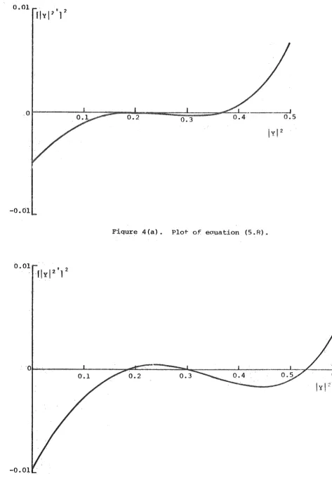
0.353, a101 = 0 •. 213. The moduli and arguments of B99 , B1oo.v

A

Btol, for the initial pertur~ation amplitude b

=

0.01, are plotted in

figure 3. The dashed curves are the complex amplitudes ·predicted by

the linearised model, including the perturbations given by equations

(4.7). The solid curves are the complex amplitudes without linearisation,

obtained by a numerical solution of the evolution equations (4.2) from

the same initial conditions as the linearised solution.

The curves for the moduli are of most interest because they have a

direct influence on the shape of the group envelope. They demonstrate

that the linearised theory fits well over the initial interval of slow

timet but in so doing predicts incorrectly that the perturbations will

continue to grow exponentially. The full solution without linearisation

shows that the moduli of these amplitudes return to a state close to

their initial state. These curves illustrate the important property

that the prediction of instability by the linearised model over shor.t

times is not applicable to the development of the wave system over

longer times. A better fit between the linearised model and the full

solution is found for the arguments of the complex amplitudes. The

nearly constant negative rate of change of these arguments corresponds

to an increase in the phase velocity of each .of the calculated wave modes.

The second e~ample described is that.for which

c

=

0.01, ko

=

100,

K = 99.8. This example has been chosen because it shows the structure

of the perturbation solution when the sideband modulation is applied at

a wavenumber which is not already present. The perturbation variables are

~

<

~

"•

~ t(

16.

eigenvalues

A

tend towards the corresponding values of Qk±0.

2 as k

tends away from ko, as in the first example. The central eigenvalues

are A_{98 • 2}

=

-0.457, A_{99. 8}.= 0.268,

\oo.

₂ = -0.263; \o1.a

=

0.441,

with the complex set -6 ><10-4 ± O.Ol6i, 3 ><10-4 J 0.0121 favouring all

six central wavenumbers 99 ± 0.2, 100 ± 0.2~ 101 ± 0.2. The two central

A A A

modulations starting from initial condition$

a

99•8

=

B100.2

=

b,

Bk±0.₂

=

0 otherwise, are

a

₉₉•

8

=

S[ (-1. 367 + 8.869i) exp i(-6 x

10-4 _{t O.Ol6i) c}2

t

+(-1.367- 8.869i) expi(-6 Xl0-4 - O.Ol6i)F:2t

+( 1.447 + 10.026i) expi( 3 ><10-4 + 0.012i)£2t

+( 1.447- l0.026i) expi( 3 Xl0-4 - 0.012i)£2t • ·. 2

- 0.355 exp1\oo.₂£ t + ••• (0.01)

l,

(4.8a)

s;oo.2

=

S[ C-1.244 - 8.962i) exp i (-6 x

10-4 _{+ 0.016i)£}2_t

+(-1.244 + 8.962i) exp i (-6 x 10-4 - O.Ol6i)£2t

+( 1.284 - 10.084i) exp i ( 3 X 10-4 + 0.012i)£2t

+( 1.284 + 10.084i) exp i ( 3 X 10-4 - O.Ol2i)£2t

1 2 7' ., 2

1

+ 1.260 expi"lo0.₂£ t - 0.33 exp1A₉₉•₈r t + •.. (0.01) •

(4.Bb)

The linearised solution could not be compared with a full solution of

the evolution equations because the large number of fractional

wave-numbers placed the calculation beyond the computing facilities availablP,

However, since the nearly resonant mechan.i.rJm of enerqy tr,msfor wi lh i 11

quartets which applied in the previous example still applies here, it

can be expected that the. above solution is valid only for an initial

interval in slow time, and that cyclic recurrence will occur over longer

1/.

5. An analytical soh~tion of 1-ho ovolution t~quations

A nonlinear wave group of small amplitude,.such as that in the

examples of the previous section, is dominated by the interactions

between its three central wave modes. The evolution equations (4.2)

are solved therefore for a nonlinear wave system consisting only of the

three central wave modes.

The coefficients in equations (4.2) are approximated and rewritten

as follows,

p

ko.

R

kQ.m

=

=

1

4 =

1

Po,

1

+-

=

pi

4 (from equation 4.3b),

B(ko£)

1

1

(from equation 2.7). 2

The time variable is changed to T

=

£2t. The three complex amplitudes

are rewritten

Bko-1 = X,

The evolution equations (4.2) then become

X' - iPtX

=

-~i{<lxl2

+

2IYI2

+

2lzl

2

>x

+

y2z•},

(S.la)

'l'

_{- iPo"i}

=

-%-i{(2lxl

2

+

IYI

2

+

2lzl

2

lY

+

2XY*Z},

(S.lb)

Z' - iP1Z

=

-%-i{<2lxl

2

+

2IYI2

+

lzP>z

+

y2x*}.

(5 .lc)

.The steady solution of these equations is the nonlinear wave group whose

amplitudes are given by

x2

=

z2

::::

-

1 _{(4 -} 1

al2

(5.2a)

(ko

£)

2

=

60

y2

= 1 ₍₁

₊

1 _}

_ao2

(5. 2b)

(ko

£) 2 =

10

Two first integrals of equations (5.1) may be found immediately.

These are

lxl

2

+

IYI

2

+

lzl

2

=

Ct,

I X

1

2

- I z I

2

-

C2 ,

(5.3a)

lB.

where Ca, C2 are constants. When the combination Y" Y* - Y*"Y is

formed and the right hand side simplified using equation (5.3a), it

may be integrated to yield

Y' Y*- Y*'Y

=

.!:.iiYI~

+ · (

1 1 3c 2

1

_J

IYI2 + ic3,

4 1

2

+ 4(ko£)7 - (5.4a)

where C3 is a real constant. This equation is equivalent to

(arg Y) • =

₈

1

I I

2 1 1 3Ct

c

3

Y +

4

+

8 (ko

E:f2" -

4

+

2l

Y 12 (5.4b)

ly 1

2'

--Next, the derivative Y'Y* + Y*'Y is formed from equation (.S.lb),

it is differentiated and the right hand side simplified from equations

I 1

2 II

(5.1a,c) and equations (5.3a,b) to yield Y ·as a cubic equation in

I Y 12• This ~ay now be integrated and written

[ IYI21

1

2 =

ao

lv 1

8 +

a.

I Y

1

6

+

o:1 I Y

I"

+ a3IYI 2 +(4

,

(5. 5)

where

ao

= 7 16 '

O.t

=

3 _ 5Ct

S(ko £) 2 4

(

1 Ct

r

₊

_{c2 - cz}

3

a2

=

-4(ko£) 2 +

2

1 2

+

2c3,

0.3

= -

_{2C 3 (}

4

(k~

£) 2 + Ct

2

J

'

and ~ is arbitrary •

. Equation (5.5) defines T as an elliptic integral of the first

kind in IYI 2 [13], which means in particular that IYI 2 is periodic in

T (

=

£2tJ. The equation may be rearranged in particular examples to

calculate the elliptic integral solution, but instead the periodicity

is demonstrated more directly by simplifying.the quartic in IYI 2• If

the initial values of X, Y,

z

are denoted by X_{0 ,} Y_{0 ,} Z₀ respectively,

equation (5.5) may be rewritten

[ I Y

1

2

'F

= -[

(I Y

1

2 - I Yo

1

2)

<il

Y

1

2

+

il

Yo

1

2 - ₄

(k~

£) 2 -

c~

>

+ XoY~2Zo +

xJ'yJzt1

2 + IYI "{ ( IYI2 - Ct) 2 -

en .

(5.6)

19.

C2

=

0 and equation (5.6) reduces to

[ I

Y

1

2

'F

=

(I

Y

1

2 -

I

Yo

1

2

)(lj

Y

I

2 +

lj

Yo

I

2 - _ _1_.., - 3 C1. ) x

4 4 4(k₀ £)' 2

liiY1

4

+

(

4

(k~s)2- c~)IYI

2

+fiYol

4

-

(

4

(k~e:)2 +

3

_~

₁

_]1Yol

₂

₁

•

(5. 7)

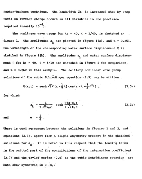
When Y satisfies the steady solution (equations 5.2), equation (5.7)

becomes

(5.8)

This equation, with ko£

=

1, is sketched in figure 4(a) as a plot of

[ IYI21

1

2 against IYI2• Necessary conditions for a physically relevant

I

solution are [ jy 12 ] 2 ~ 0 and

IY

12 ~ 0, both of which are satisfied at

the double root jyj2 = aJ = 0.2, corresponding to the steady solution

Y

=

ao.

When the steady solution with ko£

=

1 is disturbed by an initial

perturbation of the central mode, namely Xo =at, Yo= ao + 0.1,

Zo

=

at, the resulting evolution is the sa.me in essence as in the first

A

example of the previous section (where the initial perturbation b was

0.01 instead of 0.1 here). Equation (5.7) is applicable to these

initial conditions, and reduces to

(5.9)

since yJ

=

0.3. This equation is sketched in figure 4(b) as a plot of

[ jyj2

'J2

against

IYI

2• The initial point on the graph is at

IY

12

=

0.3,

IY

12'

=

O, jy 12"

<

O, from whiqh jy 12 decreases until it

reaches the point jy 12 =

~~

, jy 12' = 0, jy 12"

>

0, where IY I increases

until it returns to the initial point, and so on. Hence IYI is a

periodic function of.T ( =s2t), with a minimum value 0.43 and a maximum

value 0.55, while from equations (5.3a,b).

lxl

and

lzl

have the same

20.

rate of change of arg Y is given by equation (5. 4b), and in this example

has a mean of about -0.1.

The effect of a perturbation applifld to the nonlinear waV<.' group

is to redistribute the quartic in figure 4(a) so that it has a finite

intersection with the

IYI

2-axis in the neighbourhood of the initial

point. For a small initial perturbation, the change in height of the

quartic near the initial point is small, but because of the flat slope

of the quartic near this point, the range of

IYI

in the resulting

periodic motion may be much larger. However, the important property

is that for any small perturbation of the three wave mode nonlinear wave

group, the resulting evolution of the wave group is strictly periodic,

even though a linear stability analysis shows that the wave group is

unstable to small perturbations.

6. Numerical solution of the evolution equations

The evolution equation for Bk (equation 4.2) may be re.,Yritten as

the difference equation

~(T +i\T) - Bk(T -t.T)

2M

. Bk ( T + t. T) + Bk ( T - M) - 1. pk 2

'where T = £2t, and this equation then used to generate a stepwise

(6 .1)

numerical solution of B , k{) - k1 ~ k ~ k{)

+

k1 • This form of differencf~

k

equation was applied successfully to quadratic nonlinearities in a

previous investigation [14], and is such that the linear terms are

numerically stable • . The time step used in most calculations is

t'J.T :i: 'fT/200 •. The numerical S'Jlution described in §4 and in figure 3

...

,.

The principnl example tn be doscrlnod hon~ l!l "qonPtillin<~tlou

of tho 3 wave modC' example solved nnalytically in Uw pn,vious s<!ction.

The system is extended here to 21 wave modes, 90 ~ k

<

110, and the

calculations are started from the same initial conditions as before,

namely Btoo = a10o

+

0.1, Bk = .~ otherwise. The results are presented

in figure 5.

The moduli of B99, Btoo, and Btot are drawn in figure S(a). The

important property of this solution is that the moduli are found to be

almost periodic over the 5000 time steps of the integration, with no

evidence of a loss of periodicity beyond the interval of calculation.

The form of the solution agrees with that found in the last section for

a 3 wave mode system, but the valu~s for the amplitude and the period

of the moduli differ from those calculated because of the influence of

the additional 18 wave modes.

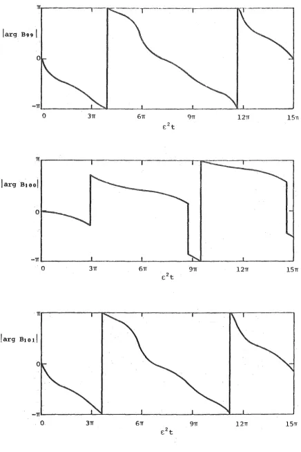
The arguments of B99 , B10o, and Bto1 are drawn in figure 5(b).

The interesting feature here is that the negative mean rate of change

of argument is nearly the same for all three wave modes, indicating that

the phase velocity of the wave inside the wave group is increased as a

result of the initial positive perturbation of the central wave mode.

Also, since the phase difference between the wave modes remains almost

zero, the change in envelope of the wave group is determined almost

solely by the change in moduli of the wave modes.

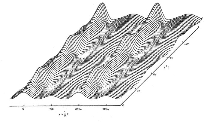
The upper side of the wave group envelope is drawn in figure 5(c)

.as a function of x and £2t, relative to an observer moving with the

propagation velocity

~of

the unperturbed wave group. The interval

r;r

slow time that is illustrated is 0 ~ £2t

<

15TI, only part of that in

figures (Sa,b). It can be seen that the. small oscillation in shape of

.the envelope is related directly to the periodic oscillation of the

22.

investigation, . that the calculated linear instability of the· nonlinear

wave group gives a false impression of the evolution of the wave group.

The behaviour of the wave group shown in this figure is the behaviour of

a

stable system, and the definition of stability that is applied to this

system should be consistent with this figure.

A comparison of figures 3(a) and 5(a) shows that the period of

oscillation of the moduli, like their amplitudes, is dependent on the

magnitude of the initial perturbation. This is to be expected for a

nonlinear system such as this, and is demonstrated by the analytical

:n.

NnnJl11t1t1t' WllVt; qru11pt1 ol ftlttutt~lll o't,llltrll WoiVt~llllllllu•i''• o111d ltttllt'ti

of different propagation veloclties, lt<wo beun shnwn t.htmrotlc:ally ,•wd

experimentally [

sl

to hav.e the soliton property that when they interact,

they emerge from the interaction with at most a change of phase. The

numerical method desc:ribed.in the previous section is applied here to

the calculation of the interaction between nonlinear wave groups of

the same and of almost the same central wavenumbers propagating in the

same direction.

The three wave mode analytical solution ( §5) may be applied to

finding the values that should be given to the amplitudes and phases

of two nonlinear wave groups of the same central wavenumber so that the

interaction between them is as large as possible. Following these

approximate calculations, the initial conditions were chosen to desc:r:ibe

a nonlinear wave group for which

e:

=

0.01, ko

=

100, superposed on a

second nonlinear wave group for which £

=

0.0075, ko

=

100, with their

envelope crests at half the fundamental wavelength apart, and their

central wave modes in phase. .The evolution of this system, calculated

for the waveband 90 ~ k ~ 110 over the interval 0 ~

e:

2t ~ 15TI, is

sketched in figure 6.

The moduli of B99, B1oor and BJoJ in figure 6(a) display excellent

periodicity over the interval calculated, even through the amplitudes .of

oscillation are much larger than in previous examples. The complex

amplitude B1oo passes through zero where there is a discontinuity of TI

in its argument. The evolution of the two envelopes is illustrated in

figure 6(c), where it can be seen that the interaction between the two

nonlinear wave groups has the form of an oscillation of energy between

them, without any significant change in their relative positions.

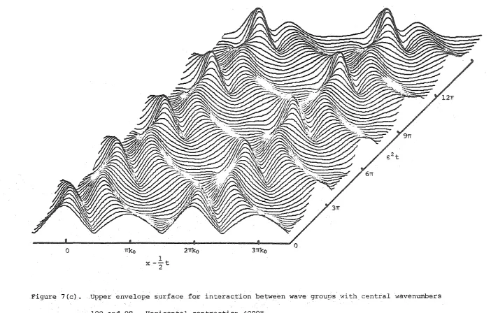
The final example calculated has the same initial conditions as in

nonlinear wave group lH ko "". 90. 'l'hn paths of thn PnV•' lnp<~H r>f Lho two

wnvetraina may bn di.AcN··ned i.n tho upper envelope t:Ut f<we j n fiq11rfl 7 (<.:).

The fanter nonlinear wave groups with central waw•nnmhet· 100 h<tve ine.lrl

paths parallel to the c2t-:axis, indicating that they are propagating

with the velocity

~of

undisturbed nonlinear wave groups at this central

wavenumber. The slower nonlinear wave groups with central wavenumber

98

have mean paths across the figure, with an exchange of roles occurring

between envelope crests as the two set.s of crests intersect. This figure

bears a striking resemblance to that describing the interaction of two

wavetrains in shallow water ([ 14], figure 4), even though the present

figure describes envelopes on deep water and the previous figure

described waves on shallow water. The immediate reason for the

resemblance is the similarity between the soliton properties of the

cubic Schrodinge:r:; equation and the soliton properties of the Korteweg

and de Vries equation. A unified approach to the complete spectrum of

nonlinear water waves·. may find deeper reasons for this resemblance~·

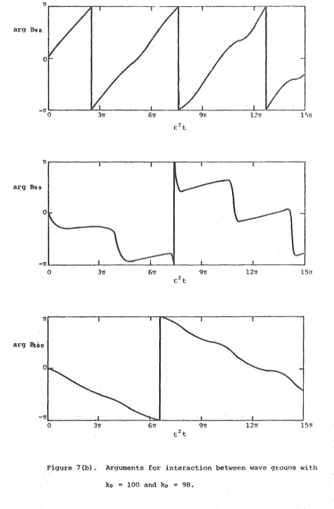
The moduli and arguments of B9s ,·B99, and Btoo are sketched in

·figures 7 (a), 7 (b) respectively, where it can be seen that the apparent

periodicity of figure 7(c) is not consistent with a closer scrutiny of

the wave modes at the centre of the interaction. The reasons for the

·loss of periodicity in this example, compared with the good periodicity

25.

8. Discussi.on

The analyaiR hr•ro hilS bc:wn reatr.ir.tc<l t:o w.:wo AI rut:t;uro~l (:nmpoBNt

of wave modes in a narrow waveband, for which tertiary interactions

between the wave modes are significant. Permanent wave structures of

this type were found to be linearly unstable, but to be stable in a

wider sense in that they exhibited a periodicity or cyclic recurrence

over longer times. These properties have been demonstrated also for

a modulated Stokes wavetrain [9], because the modulat~d wavetrain was

found experimentally to evolve into a 'pulse train' of the type

investigated here. An attempt will be made now to apply the methods

of the present investigation to modulated Stokes wavetrains, for which

the narrow waveband assumption does not apply initially; although the

cited experiments suggest that it may apply at later times. Stokes

waves are linearly unstable to sideband modulations in the same directit.

as the wavetrain on deep water, but are linearly stable to the same

modulations on shallow water. It is intended therefore to investigate

.the cyclic r'ecurrence of nonlinear water waves for the whole range of

Heforcnccs

1. D.J. Benney and A.c. Newell, The propaqation of nonlinenr wave

envelopes,

J. Math. Phys.

46,

133-139 (1967).

2. Bruce I. Cohen, Kenneth M. Watson, and Bruce J. West, Some

properties of deep water solitons,

Phys. Flu-ids.

19, 345-354

(1976).

3. V.E. Zakharov, Stability of periodic waves of finite amplitude on

the surface of a deep fluid,

J. Appl. Meoh. and Teah. Phys.

2 ~

190-194 (1968).

4. Vincent H. Chu and Chiang

c.

Mei,, The nonlinear evolution of

Stoke~ waves in deep water,

J. Fluid Meoh. 41,

337-351 (1971).

5. Hideno:d Hasimoto and Hiroaki Ono, Nonlinear modu1a tion of gravity

waves,

J. Phys. Soe. Japan

33,

805-811 (1972).

6. A. Davey, The propagation of a weak nonlinear wave,

J. Fluid Mech.

63,

769-781 (1972) •

. 7. G.B. Whitham,

Linear and Nonlinear Waves,

Wiley, 1974.

·a.

Henry

c.

Yuen and Bruce M. Lake, Nonlinear deep water waves:

Theory and experiment,

Phys. Fluids.

18, 956-960 (1975).

9. Bruce M. I.pke, Henry

c.

Yuen, Harald Rungaldier and Warren E. Ferguson,

Nonlinear deep water waves: Theory and experiment. Part 2. Evolution

of a continuous wave train,

J. Fluid Mech.

83,

49-74 (1977).

10. G. Roskes, Comments on "Nonlinear deep water waves: Theory and

27.

11. T. Brooke Benjamin and J.E. Feir, The disintegration of wavetrains

on de~p water. Pa.rt l . Theory,

.r.

F'Luid Mec•h. 27; 417-430 (1967).

12. P.J. Bryant, Stability of periodic waves in shallow water,

J.

Fluid

Meah. 66,.81-96 (1974).

13. L.M. Milne-Thomsori, Elliptic integrals,

Handbook of MathematiaaZ

Functions,

Chap 17, Ed Milton Abramowitz and Irene A. Stegun,

oover, 1965.

14. P.J. Bryant, Periodic waves in shallow water, ,J. Fluid Mech.

·!i!J,

a

2fl.

0.4 ___ ,,.- .... . ·--1-· ... _ .. - -·

+

0.3

"\. 0.2 +

+

k

0.1

0 30

+ +

+

.,

40

k

50

Figure l(a). Nave amplitudes when ko

=

40, c -· 1/40.

Figure l(b). One group wavelength (horizontal contraction 64TI) when

ko "" 40, £

=

i/40.

0.10 T I I

++

o.m~ f- +

₊

+

₊

0.06

1-+

...

-+ +

.0~04 _{1- +}

-+

+

0.()2 f-.

₊

.._+

++

0 . .&..&.4+++++ I I

20 30 40 50 60

k

· l!'igure 2 (a) • · t•'ave amJ?li tudes when k0 = 40, £ = 1/10.

oll=o-.... moe...__ ... __ ... _...._..., ... ...,,...,._,_,_,..._-..a:~- M - - = rsm

~i~ure 2(b). One grouo wavelength (horizontal contraction 16TI)

23

ttl ~ .... 0 0 ~ 0 0

-0 0 0 0 0 0 0 0 .0

--0 0

.

.

--.

.

.

.

--.

..

0

.

.

.

tv tv N :-,) w w w

....

N N ·IV ~.,) 0 N ;l)o. 0\ ;l)o. 0\ 00 0 0 lo.J

....

C' 0 0 0 ~

1-\\

-1

~~

/

1\,) ~

~

=I ~ I

I

I

'

I

I

\ I

'

\

~ ~

I

.

~

;j~\

\

\

•

,z::,. ..J

'

=I

I

I t

(T)

I

I

u

I

l

'

'

!

N (T)

'

(T)

I

rT I N

'

,.,

I

rT

'

rT

'

I

~

~

I

I

-1

~~

"

'

0\

I

I

'

=I

!

'

I !

'

•

i

'

I

1

I

30.

-0.11T

-0.21Tb---~--~---~---~·~· ---~---~

0 21T 41T 611 A1T 1o·rr

arg B100

-O.l1T

.:.;0. 21T

'---'---'---A---L---.;.__

__

_.J

0 21T 41T 61T 81T l01T

arg B1 o 1 ·

:n.

-0.01

Fiqure 4(a). Plot of ~auation (S.R).

0.01

[image:32.595.51.525.70.769.2]

12.

0.4 -~- .. T

0.3

I

8991

0.2

o.J

.

.-4

I __j_ ___ 0

0 5TI lOTI 15Tr 20TI 2511 .Q

t; 2 t

0

0.5 Cl

H ~

..

c 0 rl

0.4 .II

0

~

I

Bt 00

I

'

H

0

.

0

0.3 _w

~ (j) .c. ~ ,,.-~ r-1 ::J 'C 0.2

0 5TI lOTI 15TI 20TI 25il

£

E: ;> t

~

.0. 4 rU

L{) C.' )..I

g

·.-I ILl 0.3

1131 0 I

I

. o.

2

0 .l 1 . . - - - L - - - c L - - - ____ _l _ _ _ _ _ _ .J.___ _ _ _ _

31.

0 STI lOTI 15TI 20TI 25TI

arg BiQO

~TIL---L--~----~L-·---L----L---~---~

0 5TI lO'IT 15TI 201f 25'1[

arg B.1 o t

0

-TIL. ---~L---~---~--~L---L---~

0 5TI lOTI 15TI 20TI 25TI

Figure S(b). Arguments when £

=

0.01, ko

A

0 7Tko

1 x-2t

27Tko 37Tko

Fiqure 5(c). Uooer envelope surface when € = 0.01, ko

Horizontal contraction 40007T.

A

100, K 100, b = 0.1.

157T

...,

35.

0.6

....---.---..,---

..

·--.---.0.4

ls991

0.2

.

0 0 .-1 II 0 -~ <!)

0 ~ Ul

0 31T 61T 9rr 121r 15TI

E2t

fi

·.-4

0.9 ~

Ul o. ::l' 0 N .tr> Q) :> Ill

0.6 .~ _s:::

<!)

(!)'

Is.

oo

I

:;; .jJ (J) .0 s::: 0

0.3 .•.-4

.jJ u Ill 1-1 (J) .jJ s::: ·.-4 1-1 0 ~

0 31T 61T 9n 1211 . 151T 'H .-l

f:2t '::l _'0

0.6 .9 ,;;,

~

ro 1.0

Q) 1-1

0.4

&

·.-4

~

IBtol

I

0.2

36.

n---,

r

-larg B991

.I

0 31T 6TI 91T l2'1T

-TIL---L---~L---~~---~b---~

·a

3'1T 61T 9TI l21T l57r

-nL---~~---~---J---J-~---~~

0. 31T 61T _9TI 12'1T 15'1T

Figure 6(b). Arguments for interaction between wave groups with

[image:37.595.35.472.72.727.2]

0 ifko

1 x - - t

2

21fko 31fko

Figure 6(c). Upper envelope surface for interaction between wave grouPs with same ko

=

100

[image:38.842.74.754.78.484.2]

3H.

O.Gr---~---~---,---~---l

8_9fl

I

OJ

.

01 0 .!<! '\.1 ~ <0 c c r-i

q

0

0 3'1T 61T 91T l2'1T lSTI ~

f.:2t .c.

+l

·rl

0;.6 ~

Ul p. ;::1 0 I>; tJ (!; ~ 10

0.4 :;:

~

<I) <I)

~

+l

18991

<I)

.Q

r::

0

o.·2 ·rl _+'

0 ro H .I)) +l c ·rl H 0 4-l 0 ·rl

0 3'1T 6'1T _£2t 9'1T 12TI l5'TT r-1

;::1

'd

0

0.6 ~

ro ~ !'-<I) ·H ;::1

0.4 b

'•.-1

j:L,

18100

I

0.2

arg B9s.

arg B99

0

-n~---~---~---L---L---~---~

0 3n 6n 9n 12TI l5'1T

n

arg .Btoo ·

-TI~---._---~~~---L---~---J _{0 3TI 6TI 9TI 12TI 15TI}

Figure 7(b). Arguments for interaction between wave grouos with

[image:40.595.36.513.99.824.2]

Figure 7(c).

1

x - - t

2

Upper envel ope surfa _{·. . ce} for .

[image:41.842.55.757.72.520.2]

PREVIOUS Ml\TIIEMJ\'riCJ\ I, RESP.l\RCH REPORTS

1. (November 1976) BRYANT, P.J. (Reprinted March 1978) Permanent wave structures on an open two layer fluid.

2. (December 1976) WEIR, G.J.

Conformal Killing tensors in reducible spaces.

3. (January 1977) WEIR, G.J. & KERR, R.P.

Diverging type~o metrics.

4. (February 1977) KERR, R.P. & WILSON, W.B.

Singularities in the Kerr-Schild metrics.

5. (May 1977) PETERSEN, G.M.

Algebras for matrix limitation.

6. (August 1977) GRAY, A.G.

Topological methods in second order arithmetic.

7. (September 1977} WAYLEN, P.C.

Green functions in the early universe.

8. (November 1977) BEATSON, R.K.

The asymptotic cost of Lagrange interpolatory side conditions.in the space C(T).

9. (November 1977) BEATSON, R.K.

The degree of monotone approximation.

10. (November 1977) BREACH, D.R.

On the non-existence of 5-(24,12,6) and 4-(23,11,6) designs.

11. (February 1978) BRYANT P.J.

&

LAING A.K.

Permanent wave structures and resonant triads in a layered fluid.

12. (August 1978) BALL, R.D.