Portfolio Performance on Agency Mechanism with Capability of Manager

(1)

ISSN Online: 2162-2086 ISSN Print: 2162-2078

DOI: 10.4236/tel.2018.81002 Jan. 4, 2018 28 Theoretical Economics Letters

Portfolio Performance on Agency Mechanism

with Capability of Manager

Haijun Yang, Wei Xia, Jian Fu

School of Economics & Management, Beihang University, Beijing, China

Abstract

By given different capabilities of managers, a novel model of optimal con-tracting is proposed in agency problems, which adds a new variable denoted by the manager’s ability in delegated portfolio management. Then we com-pare our results with Dybvig and Farnsworth’s (2010) and find a new effect by appending this variable. The results show that in the first-best situation with log utility, the optimal contract is in accord with the result of Dybvig and Farnsworth’s (2010). In the second-best situation, the optimal contract is a proportional sharing rule plus a bonus. However, the bonus is associated with variables including private signals and the manager’s ability. In the third-best situation, the manager’s share is no longer a constant; and the manager’s fee is no longer a linear combination of the returns, which depends on the signal and the manager’s ability. So manager’s ability is an important variable for the market return. We can also find that these institutional features are more sim-ilar to practice than other existing agency models and consistent with the real-ity of the situation. The numerical results also verify the solutions.

Keywords

The Ability of the Manager, Asymmetric Information, Moral Hazard, Optimal Contraction, Private Information

1. Introduction

Principal-agent theory studies internal problems of corporations from a pers-pective on agents’ asymmetric information, inconsistent interests and uncertain behaviors. It includes incentive mechanism and risk-shared problems, which are getting a lot of attention [1]-[6]. When the traditional economics fails to explain the internal problem of corporation, economists just go down two different ways to study the delegated problem which prevents the internal operation of compa-How to cite this paper: Yang, H.J., Xia, W.

and Fu, J. (2018) Portfolio Performance on Agency Mechanism with Capability of Manager. Theoretical Economics Letters, 8, 28-47.

https://doi.org/10.4236/tel.2018.81002

Received: October 27, 2017 Accepted: January 1, 2018 Published: January 4, 2018

(2)

DOI: 10.4236/tel.2018.81002 29 Theoretical Economics Letters ny, so it leads to two approaches: empirical research and standard one. Empirical agency theory is characterized by intuition, with emphasizing on analysis for drawing a contract and controlling the social factors, focusing on describing the control mechanism of the limits of agents for pursuit of self-interest. Standard agency theory is characterized by use of formal mathematical models, and clari-fying accurate information assumptions required by diverse models. Then it tries to explore the incentive and risk allocation mechanisms between the principals and agents, and also desires to point out that a contract is valid on behaviors of a contract with asymmetry information and uncertain results.

Mirrlees [7] presented two kinds of models for a productive organization. In the first, both productions and rewards are based on the performance of indi-viduals, which are perfectly observed, but their abilities are not observable. The second model, which focuses on the imperfect observation of performance, shows optimal payment schedules and organizational structures. The innovation of this article is to introduce time cost when principals observe the performance of agents. Then, Cox and Huang [8] got that for the first-best problem with posi-tive initial wealth, they presented in essence a portfolio optimization, and an op-timal solution under an asymptotic marginal utility and growth bounds on the tail probabilities of a state-price density. Holmstrom [9] pointed out the easiest way to solve moral hazard problem by investing resources into monitoring and use this information in a contract. He studied importance of non-linear con-tracts in the incentive mechanism and analyzed three optimal concon-tracts. He got results that when the payoff alone is discernible, optimal contracts are second-best due to a moral hazard problem. Myerson [10] employed Bayesian viewpoint to study collective choice problems. It is shown that a set of expected utility allocations which are feasible with incentive-compatible mechanisms is compact and convex, and the set of expected utility allocations includes the equi-librium.

Grossman and Hart [11] addressed that the optimal way of implementing an action with agents could be found by solving a convex programming problem, when the agents’ preferences over income lotteries were independent of the ac-tion. The purpose of this paper is to develop a method for analyzing the princip-al-agent problem which avoided difficulties of the “first-order condition” ap-proach. Rogerson [12] announced that sufficient conditions of the first-order approach and pointed out that the Pareto-optimal wage contract was non-decreasing in output under these conditions. Hart and Holmstrom [13]

made a survey of the agency theory. They divided this problem into two situa-tions: one is that agents’ actions can not been observed; the other one is that agents’ actions can be observed.

(3)

DOI: 10.4236/tel.2018.81002 30 Theoretical Economics Letters Kihlstrom [15] considered the situation is one in which a securities analyst provides an investor with information about the return on a risky asset which they interpret as the market portfolio. In a moral hazard setting, the investor would like to pay the analyst a fee that depends only on the level of effort he ex-erts. In an adverse selection setting, the investor knew the analyst’s ability, and the investor would be able to avoid paying for the useless information provided by an analyst who lacked ability, and he would also be able to pay the able ana-lyst a fixed fee in a linear form of the contract.

Admati and Pfleiderer [16] proposed a new assumption which used a bench-mark portfolio of risky assets, for example, index funds that cannot be simple ra-tionalized. In this article they analyzed effects of benchmark-adjusted compen-sation in theory. Specifically, they examined whether a portfolio manager can be induced to choose the optimal portfolio for investors through the use of bench-marks and whether benchbench-marks might help in solving various types of contract-ing problems that potentially exist when investors delegate investment decisions to a portfolio manager. They also found that benchmarking provides no incen-tives for efforts. Stoughton [17] got the similar results with the Admati et al.[16]. The difference is that this paper investigated the significance of nonlinear con-tracts on the incentive for portfolio managers to collect information. In addition, the manager must be motivated to disclose this information truthfully. They analyze three contracting regimes: first-best where effort is observable, linear with unobservable effort, and the optimal contract within the Bhatta-charya-Pfleiderer quadratic class. They found that the linear contract leads to a serious lack of effort expenditure by the manager. This underinvestment prob-lem can be successfully overcome through the use of quadratic contracts. These contracts are shown to be asymptotically optimal for very risk-tolerant princip-als.

(4)

Simi-DOI: 10.4236/tel.2018.81002 31 Theoretical Economics Letters larly, Basak, Pavlov and Shapiro [20] showed that restricting the deviation from a benchmark can reduce the perverse incentives of an agent facing an ad hoc convex objective. They attempted to isolate the two most important adverse in-centives of a mutual fund manager: an implicit incentive to perform well relative to an index, and an explicit incentive to manage the fund in accordance with her own appetite for risk.

Almazan [21] deliberated the constraints on the managers of the mutual fund. The constraints includes boards contain a higher proportion of inside directors, the portfolio manager is more experienced, fund is managed by a team rather than an individual, and the fund does not belong to a large organizational com-plex. Then they used the data of American mutual fund to verify the income of the fund is not affected by the investment restrictions.

Laffont and Martimort [22] made a survey of the theory of incentives. This ar-ticle studied from the basic model to the rent extraction-efficiency trade-off, in-centive and participation constraints, moral hazard model, mixed models, dy-namic models and generalized agency models. They assumed these models re-spectively and indicated the model construction and the subsequent extension of some restrictions. In these models, they used the variable of the type of the manager. They also studied from two types of the managers to a variety types of the managers. They obtained the optimal contract by the game method.

Dybvig and Farnsworth [2] studied the portfolio performance on the agency. They used three variables including market states, the manager’s effort and the private signals, and got the results of the optimal contract and the payoff to the agent. The three optimal contracts contains first-best contract (the manager’s effort and the private signals can be observed), second-best contract (the signals can be observed, but the manager’s effort cannot be observed), the third-best contract (neither the effort nor the private signals can be observed). This article got the results that in a first-best situation, the optimal contract is a proportional sharing rule. In a second-best situation, the fee appears as a proportion of the managed portfolio plus a share of the excess return of the portfolio over a pas-sive benchmark portfolio. In a third-best situation, such excess return strategies will provide incentives to work but will tend to make the manager overly con-servative.

Xu [23] made summaries of the relevant research of the relationship between principal and agent and pointed that future research can combine governance mechanism with some methods to solve these questions in order. Cai [24] ex-tended the classic principal–agent problem to the implications of uncertainty in demands of agents on the principal’s contracts. They studied the special case that two distributions each take two discrete values and showed analytical solutions derived from numerical solutions for it.

(5)

DOI: 10.4236/tel.2018.81002 32 Theoretical Economics Letters compensation of portfolio managers is an enduring subject of question among practitioners and regulators. Performance measurement has very strong rela-tionship with optimal managerial contracting, but the academic literature has mostly considered two questions individually. The most existed researches con-cern the agency problem are based on the market states, signals states and man-ager’s effort, there are few research and prediction on introducing the variables of the manager’s ability. This paper will try to do some studies on introducing the variables of manager’s ability to solve the optimal contract in different con-ditions. The above literatures are all not mentioned managers’ ability on agency problems. The manager’s ability is a very important variable to describe the op-timal managerial contracting, which can be measured by historical recorder of the manager. The manager’s ability cannot be replaced by the manager’s effort, but they have very strong relation. The former can be exactly graded by histori-cal recorder, but the later cannot be accurately histori-calculated.

The remainder of the paper is organized as follows: Section 2 introduces the agency problem; Section 3 presents analytical solutions in the first-best and second-best cases, and discusses the problems for the third-best case; Section 4 presents numerical results in three cases; we provide summary and key conclu-sions in Section 5.

2. The Agency Problem

In this paper, a contract problem is considered between an investor and a port-folio manager. Through the contract problem, we want to find out an optimal solution without pre-assuming that the contract has any particular form or agrees to known institutions. In this way, we can compare it with the practice or other contracts supposed by other researches. It also meets the realistic market conditions in intuition. Different technologies are employed to manage informa-tion problems by different scholars. But our research tries to find out what can be done if we only use contracting and communication, which is same as the as-sumption of Dybvig and Farnsworth [2]. We present this in the typical format widely used in agency problems. And in the signal reporting stage, we grant for a direct mechanism [1] [2]. About the manager’s ability, we take it as a special component of information. The assumptions of the model are as follows:

Market returns. The market is complete and investments are made over states distinguished by different security prices. Let ω∈ Ω denote a state and let p

( )

ω _{represent the pricing density for a claim which pays a dollar in state}

ω

. In our model, the payoffs can only be happen only once, because it is a sin-gle-period model. Then we assume that there are many small agents in a finan-cial market, and they are all price takers whose trades do not affect market prices. Information technology. The costly effort is denoted by ε∈

[ ]

0,1 _{, and let}

[ ]

0,1

A∈ _{denote the manager’s ability. For getting a simple form of the solution,}

(6)

DOI: 10.4236/tel.2018.81002 33 Theoretical Economics Letters

(

)

(

) (

)

(

)

(

)

(

)(

) (

)

1 2

3

, ; , , 1 1 ,

1 1 ,

f s A Af s A A f s

A f s

ω ε ε ω ε ε ω

ε ω

= +_ − + − _

+ − − (1)

Equation (1) is the probability density of the signal s and the market state. Here, f1 and f2 is an “informed” distribution and f3 is an “uninformed” distribution. The difference between f1 and f2 is that the market state

ω

must be different. Because if we suffer from a financial crisis, the manager has strong ability and try his best, he also can get more market return. Then s and

ω

are assumed independent in f3, i.e., f s3

(

,ω

)

= f s f

( ) ( )

ω , the marginal distributions’ product. f s

( )

and f

( )

ω _{are all marginal distributions, and} for the informed distribution, they are assumed to be the same. For

ω

, the manager’s effort choice and the manager’s ability will influence the market return.

The manager cannot distinguish form two kind information: one is the signal observed and another is the signal unobserved. Nevertheless, the manager knows that his ability and effort have very strong relation with an informative signal. More effort and ability are paid out, more informative signal are likely gained. Using the mixture model will not lose generality if there are only two effort and ability levels and it helps use the first-order approach in many agency models.

Preferences. In this paper, logarithmic Von Neumann-Morgenstern utility functions are used to describe the utility of the manager and the investor, meanwhile, the manager also burdens a utility cost of his ability and expanding effort. If his ability is a high level, the cost of his effort is less. It is different from the preferences of Dybvig et al. [1]. Respectively, we denote log

( ) (

φ −c ε,A

)

_as

the manager’s (agent’s) utility, where

φ

_{is denoted for the manager’s fee and}

(

,

)

c ε A is denoted for the cost of the ability and the effort. In this paper,

(

,

)

c ε A _{is assumed differentiable and convex,}c′

( )

0 =0_{and all the problems}

have optimal solutions [2][5][15]. log

( )

V is the utility of the investor (prin-cipal), where V is the value of remain in the portfolio after pays the fee. u si

(

,ω

)

is denoted for the utility level log

( )

V prearranged s and

ω

, and we use

(

,

)

m

u sω _{to indicate the equilibrium utility level of manager. The wealth is} de-noted as log

( )

φ with certain s and

ω

.

Initial wealth and reservation utility. w0 is the investor’s initial wealth, and the manager is assigned without any initial wealth. Under the restriction of the manager’s reservation utility level of u0, agency problems try to maximize the investor’s utility.

(7)

DOI: 10.4236/tel.2018.81002 34 Theoretical Economics Letters the manager’s choice of portfolio-strategies as a reflection of the signal, and the truthful reports can promote manager to work harder.

There are three restrictive conditions: the budget constraint, incen-tive-compatibility of the choices intended and the manager’s reservation utility level. Our goal is to find out an optimal solution under above mentioned three restrictions. Then, three forms (the first-best, the second-best and the third-best) of this problem need to be solved. In this paper, the manager’s ability can be measured for below three situations. Furthermore, the first-best assumes that both the manager’s action and portfolio can be observed, which mean that the financial market is a competitive one with a competitive allocation and can be taken as a benchmark; for the second-best, the information signal can be ob-served and the effort cannot be obob-served, but the manager wants to do his best to choose the effort; for the third-best, both the signal and the effort cannot be observed, which makes it more difficult than the second-best.

First-best. Use the u si

(

,ω

)

, u sm

(

,ω

)

,

ε

and A to maximize investor’s expected utility.

(

)

( )

(

) (

)

(

)

( )

(

)(

) ( ) ( )

1 2

, d d

, 1 1 d d

i

u s Af s f s s

u s A A f s f s s

u s A f f s s

ω ε ω ω

ω ε ε ω ω

ω ε ω ω

+ _ − + − _ + − −

∫∫

(2)

The budget constraint is

(

∀ ∈s S

)

∫

(

exp

(

u si

(

,ω

)

+exp

(

u sm

(

,ω

)

p

( )

ω ω ωd = 0 (3) The participation constraint is

(

)

( )

(

) (

)

(

)

( )

(

)(

) ( ) ( )

(

)

1 2 0

, d d

, 1 1 d d

, 1 1 d d ,

m

u s Af s f s s

u s A f f s s c A u

ω ε ω ω

ω ε ε ω ω

ω ε ω ω ε

+ _ − + − _ + − − − =

∫∫

(4)

Second-best. We add the incentive-compatibility of effort:

(

)

( )

(

) (

)

(

)

( )

(

)(

) ( ) ( )

)

(

)

1 2

arg max , d d

, 1 1 d d

, 1 1 d d ,

m e

m

u s Af s f s s

u s A f f s s c A

ε ω ε ω ω

ω ε ε ω ω

ω ε ω ω ε

′ ′ = ′ ′ + _ − + − _ ′ ′ + − − −

∫∫

(5)

Third-best. As an alternative of Equation (5), append the constraint for si-multaneous incentive compatibility of effort and the requirement for truthfully reporting signals:

{ }

_{ _{( )}_}

(

( )

)

( )

(

)

(

)

(

)

( )

(

)

(

)(

) ( ) ( )

)

(

)

1 , 2

, arg max , d d

, 1 1 d d

, 1 1 d d ,

m e s

m

s u s Af s f s s

u s A A f s f s s

u s A f f s s c A

ρ

ε ρ ω ε ω ω

ρ ω ε ε ω ω

ρ ω ε ω ω ε

′ ′ = ′ ′ + _ − + − _ ′ ′ + − − −

∫∫

(6)

(8)

DOI: 10.4236/tel.2018.81002 35 Theoretical Economics Letters contingency

(

s,ω

)

_{. After given the effort level}

ε

_{, we can computed the} ex-pected utility (objective function) in each contingency through the investor’s utility level and the joint distribution of s and

ω

_{. The utility of agent should not} be smaller than the reservation utility level u0. It’s what the participation con-straint means. As for the budget concon-straint, we computes the investor and man-ager’s consumption levels according to their utility levels and then using the pricing rule ρ ω

( )

to values them. The consumption levels cannot exceed w0, which is the initial portfolio value. Because of the purely private signal and the “small investor” assumption, the manager will not affect pricing, and the pricing rule ρ ω

( )

does not change for each s.

Given a effort choice, a manager’s ability, the manager’s signal and payoff, we can find that the solution to the problem is essentially just the investor’s optimal payoff. So we can use the following lemma [2] to help reduce the number of both choice variables and constraints. By the lemma we can eliminate the variable

(

,

)

i

u sω _{and the variable will be used as the objective function of the investor’s} indirect utility, which is the optimal payoff of the investor given the variables mentioned above.

Lemma 1. In solving investor’s problem’s three forms, condition on s, the ex-pected utility of the investor is

( )

(

)

(

)

( )

(

)(

) ( )

1 2

log log 1 1

1 1

i B s

Af s A A f s

A f

ε ω ε ε ω

ρ ω

ε ω

 

 ₊ _ ₊_ ₋ _{+ −} _

    

 

 

+ − − _

(7)

where B si

( )

=ω0−

∫

exp

(

u sm

(

,ω ρ ω ω

)

( )

d .

Represents for the budget share of investor. Then we can use the original ob-jective in these problems to replace the indirect utility function.

Proof. Only in the Equation (2) and in the Equation (3) we can find the in-vestor utilities u si

(

,ω

)

. Therefore, we must solve the sub-problem of

maximiz-ing (2) subject to (3) to get the solution. The first-order condition of this prob-lem is

( )

(

)

(

)

( )

( ) (

)(

) ( ) ( )

( ) ( )

(

)

1 1 1 2 1 1

exp ,

B i

Af s A A f s f s A f f s

s u s

ε ω ε ε ω ε ω

λ ρ ω ω

 +_ − + − _  + − −

 

= (8)

where λB

( )

s denotes the budget constraint. Then we integrate the equation above with respect to

ω

, and rearrange

( )

B

i

f s s

B s

λ = ₍₉₎

Then substitute above back into the Equation (8), the first-order condition to Equation (7).

(9)

( )

(

)

(

)

( )

(

)

( )

(

)(

) ( ) ( )

1 0 1 1 2

1 1

p

R Af s A A f s

A f

ε ω ε ε ω ρ ω

ε ω ρ ω

≡ + _ − + − _

+ − − (10)

Suppose an investor does not observe s, and then a related gross portfolio re-turn is optimal for her.

( )

B f

R ≡ _{ρ ω}ω ₍₁₁₎

This portfolio will be the benchmark portfolio, because benchmark portfolios will be sensible passively managed portfolios in practice.

We also divided the signal return into two parts.

( )

1

( )

1I

f s

R s ≡ _{ρ ω}ω ₍₁₂₎

( )

2

( )

2I

f s

R s ω

ρ ω

≡ (13) The optimal return of investor is

(

)

(

)

(

)(

)

1 1 1 2 1 1

P I I B

R =εAR +_ −ε A+ −A ε_R + −ε −A R (14) Using lemma 1, the expected utility of investor can be calculated as

( )

(

)

( )

(

)

(

)

( )

(

)(

) ( )

( )

(

)

(

)

( )

(

)(

) ( )

(

)

1 2 1 2

log d d

1 1 1 1

log

1 1 1 1 d d

i i

U B s f s s

Af s A A f s A f

Af s A A f s A f s

ω

ρ ω

ε ω ε ε ω ε ω ω

=  +_ − + − _ + − −  + _ _   ⋅ +_ − + − _ + − −

∫∫

(15) As for the second term, which is denoted by K

(

ε,A

)

, depends on effort 2

ε

and manager’s ability A, but has no relation with the manager’s utilities. So we do not consider this term when dealing the problem.

3. Optimal Contracts

Now the solution to these three problems will be described blow. Firstly, we be-gin with the first-best, the simplest problem.

First-best. When a contract is first-best, the manager and the investor will share the optimal risk. For all states, the investor’s the marginal utility should be proportional to the manager’s.

The first-order condition for um is

( )

(

)

( )

{

( )

(

)

(

)

( )

}

(

)(

) ( )

1 2 exp , 1 1 1 1 m R i R u s

Af s A A f s

B s

A f ω ρ ω

λ ε ω ε ε ω

λ ε ω

= +_ − + − _

+ − −

(16)

where λR is the Lagrange multiplier. We can multiplying Equation (16)’s both sides by B si

( )

and integrate them with respect to

ω

. Then we will obtain

( )

m R i

(10)

DOI: 10.4236/tel.2018.81002 37 Theoretical Economics Letters Since the sum of the two budget shares must equals to ω0, we obtain

( )

0

1

i

R

B s = ω_λ

+ (18) From with we obtain

(

)

( )

(

)

(

)

( )

(

)(

) ( )

( )

1 2 0 ,

1 1 1 1

log 1 m R R u s

Af s A A f s A f

ω

ω λ

λ ρ ω

 +_ − + − _ + − − 

= _ _

+

 

(19) And we can calculate the manager’s fee:

(

_,

)

0

1

P R

R

s ω λ R

φ ω

λ =

+ (20) Since u sm

(

,ω

)

=log

(

φ

(

s,ω

)

. From the equation, we can find that in when

the world is first-best, there is a sharing rule that gives the manager a fixed part of the portfolio’s payoff. And it is independent with the signal. Compared with the results of Dybvig and Farnsworth [2], they are the same. The manager’s payoff is independent on the manager’s ability.

Second-best. When the contract is second-best, investor cannot observe effort, so the contract should be incentive-compatible. We also use the first-order ap-proach proposed by Holmstrom [6] and substitute condition (5) of the effort in-centive-compatibility with the following equation which is the first-order condi-tion for the maximizacondi-tion of manager:

(

)

( )

(

) ( )(

) ( )

(

)

1 2

, 2 d d

, 1 d d , 0

m

u s Af s Af s f s s

u s f A f s s c A

ω ω ω ω

ω ω ω ε

 − 

 

′

+ _ − _ − =

∫∫

(21)

Proof. Now we transform the problem to first-order version, the first-order condition of investor for u sm

(

,ω

)

is

(

)

(

)

( )

{

( )

(

)

(

)

( )

}

(

)(

) ( )

( )

( )(

)

1 2 1 2 exp , 1 1 1 1 2 1 m R i R u s

Af s A A f s

B s

A f

Af s Af s f A

ε ω ρ ω

λ ε ω ε ε ω

λ ε ω

λ ω ω ω

= +_ − + − _

+ _ − − _

 

+ _ − + − _

(22)

where λε is the Lagrange multiplier on the IC-effort constraint. Then we deri-vate it as in the first-best case, we can obtain:

(

)

( )

(

)

(

)

( )

(

)(

) ( )

{

}

( )

( )(

)

( )

0 1 2 1 2 , log 1

1 1 1 1

log 2 1 R m R R u s

Af s A A f s A f

Af s Af s f A

ε

ω λ ω

λ

ρ ω

λ _ω _ω _ω

(11)

DOI: 10.4236/tel.2018.81002 38 Theoretical Economics Letters Equivalently, the manager’s fee is denoted as following equation:

(

,

)

m p

(

P

(

) ( )

2I B

(

1

)

R

s B R λε R A R s R A

φ ω ε

λ ε

 

=  + − + + − 

  (24)

From the equation, we can find that in the second-best contract, the manager will receive a “bonus”. This bonus is related to the private signal and the manag-er’s ability. The result is different from the ones Dybvig and Farnsworth [2] get (the bonus is proportional to the sum of the excess return of the fund and a frac-tion of end-of-period assets under management).

Third-best. As for the third-best, it should also be incentive compatible to truthful report he signal. However, if the function of cost is sufficiently convex, the first-order approach can be applied and the joint effort and the constraint (6) of reporting incentive compatibility will be replaced with the first-order condi-tion for the manger’s effort, Equacondi-tion (21), and with the following equacondi-tion, which is the first-order condition to choose report choice, evaluated at

( )

s s

ρ = _:

(

)

(

)

{

( )

}

( )

(

) ( ) ( )

( )

(

) ( )( ) ( ) ( )

1 2 , d ,

1 1 d

,

1 1 d 0

m

m u s

s S Af s f s

s u s

A A f s f s

s u s

A f f s

s ω

ε ω ω

ω

ε ε ω ω

ω

ε ω ω

∂ ∀ ∈ ∂ ∂ + _ − + − _ ∂ ∂ + − − = ∂

∫

(25)

Then we can calculate the first-order condition of investor for um

(

)

(

)

( )

(

)

(

)

( )

(

)(

) ( )

{

}

( )

( )(

)

( )

{

( )

(

)

(

)

( )

(

)(

) ( )

}

( )

{

( )

(

)

( )

(

)

( )

}

1 2 1 2 1 2 1 2 exp ,

1 1 1 1

+ 2 1

1 1 1 1

1 1 m i R s s u s B s

Af s A A f s A f

Af s Af s f A

s Af s A A f s A f

Af s A A f s

s

s ε

ω ρ ω

λ ε ω ε ε ω ε ω

λ ω ω ω

λ ε ω ε ε ω ε ω

ε ω ε ε ω

λ = +_ − + − _ + − −  − + −    ′ − +_ − + − _ + − − ∂ +_ − + − _ − ∂ (26)

(12)

DOI: 10.4236/tel.2018.81002 39 Theoretical Economics Letters Equation (28) indicates that in the third-best situation, the manager’s propor-tion of the budget is variable, this is the same with it in the second-best, and the difference is that the proportion in the third-best usually depends on the signal. This partly helps induce truthful reporting. In addition, we can see from Equa-tion (26)’s the final term that even we solve it condiEqua-tional on the signal, the manager’s fee is not a linear combination of _Rp_and _RB_{, but an additional} payoff is contained in the fee.

4. Numerical Results

According to the above results obtained, we can find that in the first-best situa-tion with log utility, the optimal contract is as same as the original model. It is a proportional sharing rule over the portfolio payoff. In a second-best situation, the optimal contract is a proportional sharing rule plus a bonus. But the bonus is associated with variables including private signals, manager’s effort and the manager’s ability. In the third-best situation, the manager’s share is no longer constant, and the manager’s fee is no longer a linear combination of the returns

p

R and _RB_{. It depends on the signal and the manager’s ability. These} conclu-sions are consistent with the actual situation of financial markets. In three forms of the contract, the manger’s optimal utility is associated with variables includ-ing private signals, manager’s effort, market state and the manager’s ability. Therefore, we will turn to make the numerical results to compare the different forms of the contract. We will use the Matlab to illustrate above results. To high-light the manager’s ability effects, we will compare the results for the contract either has the manager’s ability or not.

Basic parameters. Before adding the manager’s ability, we assume that w and

s obey the conditional joint normal distribution, and correlation ρ will be pos-itive under the “informed” distribution and negative under the “uninformed” distribution. w and s’s marginal densities are the same both under the informed and under the uninformed. We use n

( )

⋅ ⋅ ⋅; , to denote the normal density by mean and variance. Then in either case the density of s is _{f s}s

( )

₌_{n s}

(

_;0,_σ2

)

_, and in the uniformed case _{f w}w

( )

₌_{n w}

(

_;0,_σ2

)

_{is density of the market state}_w_, no matter in the conditional case nor unconditional case. And in the informed case, when given s and the market state w, the conditional density is

( )

(

_{; ,} 2

(

₁ 2

)

I

f w s =n w sρ σ −ρ . We can find the risk-neutral probabilities and then multiply by the discount factor to get the state prices as

( )

_e r

(

_; _, 2

)

p w ₌ − n w r₋µ σ _{, the prices are consistent with Black-Scholes. In these} equations, r is the risk-free rate, µ_{represents the market’s mean return, and}

σ

_{denotes the standard deviation of the mean return. We can assume the mean} of signal s is 0 and the variance of s is the same as the log of market return with-out losing generality, The parameter values are set as

µ

=0.1_, σ =0.2_,

0.5

ρ

= _, r=0.05_, w₀=100_{. In order to facilitate the comparison, we adjust}

(13)

DOI: 10.4236/tel.2018.81002 40 Theoretical Economics Letters obvious distinction among three kinds of contracts because higher equilibrium effort will make the signal more informative and therefore imply more aggres-sive portfolios for manager and investor. By fixing the same optimal effort, we let the addition of the IC constraints become the only reason for the differences among different contracts. We used the way which Dybvig used. We vary the cost function to make u c0+

( )

ε =0.955 when the equilibrium effort level is chosen as ε =0.5.

When adding the variable of manager’s ability, the “informed” distribution is divided into two parts f1 and f2. Assume correlation ρ1 under the f1 dis-tribution and ρ2 under the

2

f distribution. According to the model, we can know that ρ1>ρ2. In order to get the effect of the correlation to the model, we assume the parameter values for two groups: ρ1=0.5,ρ2=0.25 and

1 0.75, 2 0.5

ρ = ρ = _{. We get expressions:}

( )

(

2

(

2

)

1 ; 1 , 1 1

f w s =n w sρ σ −ρ _and

( )

(

2

(

2

)

2 ; 2 , 1 2

f w s =n wρ σs −ρ . The cost function has changed to c

(

ε,A

)

. We also use the way which Dybvig used to change the cost function. Because of

(

0,1

]

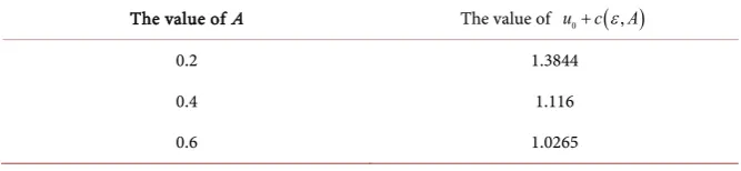
A∈ _{, we assume} A has three values, 0.2, 0.4, 0.6. We also can get the val-ues of u0+c

(

ε,A

)

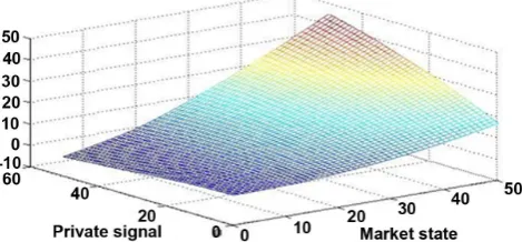
. The parameters cab be found in Table 1.

First-best. Before adding the manager’s ability, we use the original model re-sult and Matlab software to get Figure 1.

Not surprisingly, the figure shows that when states of signal and market are both high, the manager’s utility is larger. It also shows that a longer position is optimal if the signal states are higher in the market.

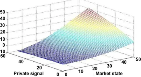
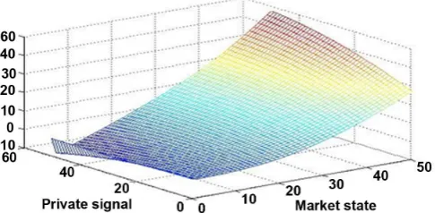
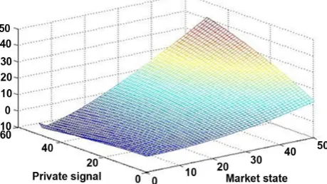
When adding the variable of manager’s ability, we use new model result and different values of manager’s ability to get Figures 2-4.

From the above three figures, we can find that the relationship between the manager’s utility and the private signal and market state is similar to the original model, higher signal and market states means larger manager’s utility. Compar-ing the three figures, it indicates that for higher manager’s ability, the manager’s utility is larger. So we can find that the manager’s ability has the important effect on the manager’s utility in the first-best situation.

Then we change the value of the correlation to ρ1=0.75,ρ2=0.5. When

0.2

A= , get Figure 5.

[image:13.595.206.540.647.724.2]

Figure 5 shows that for higher correlation, the manager’s utility is larger. We also find that for higher correlation, the manager’s utility rise more quickly than the lower correlation. We can also get the same conclusion in the second-, third-best situation.

Table 1. Basic parameter value.

The value of A The value of u c0+

( )

ε,A

0.2 1.3844

0.4 1.116

(14)

[image:14.595.257.489.74.201.2]

[image:14.595.257.491.243.366.2]

Figure 1. Manager’s utilities: Original first-best contract.

Figure 2. Manager’s utilities: first-best contract (A = 0.2).

Figure 3. Manager’s utilities: first-best contract (A = 0.4).

[image:14.595.258.492.409.531.2] [image:14.595.258.494.574.702.2]

(15)

[image:15.595.254.497.75.194.2]

Figure 5. Manager’s utilities: first-best contract (ρ1=0.75,ρ2=0.5).

Second-best. Before adding the manager’s ability, we use the original model result in the second-best situation and Matlab software to get Figure 6.

Figure 6 shows the similar conclusion to the original model in the first-best contract, which is that the manager’s utility is proportional to signal and market states. From the solution, we can get that the manager can get a “bonus” to mo-tivate them to do their best in the second-best contract. So we can find that the manager’s optimal utility in the original second-best contract is higher than the one in the original first-best contract in the other conditions being equal. This is consistent with the situation of financial markets.

When adding the variable of manager’s ability, we use new model result and different values of manager’s ability to get Figures 7-9.

From the three figures, we can find that in the second-best contract, the con-clusion does not change, the higher states of signal and market, the larger man-ager’s utility.

From the solution of the new model, we can find that the manager can get a “bonus” to motivate them to do their best. And the bonus is associated with va-riables including private signals and the manager’s ability. The figure also shows that the manager’s utility in the new second-best contract is higher than the ones in the new first-best contract under the other conditions being equal. Compar-ing the three figures, we can find out the same conclusion with that in the first-best situation, the manager’s ability has the important effect on the manag-er’s utility in the second-best situation.

Third-best. Before adding the manager’s ability, we use the original model result in the second-best situation and Matlab software to get Figure 10.

Figure 10 shows that the relationship between the manager’s utility and the private signal and market state is similar to the original model in the first- and second-best contract. From the solution of the original model, we can find that the manager can get a earning to motivate the manager to report the signal truthfully. We can also find that if the other conditions are equal, the manager’s optimal utility in the original third-best contract will be higher than the one in the original second-best contract.

(16)

[image:16.595.259.490.77.208.2]

[image:16.595.255.489.249.369.2]

Figure 6. Manager’s utilities: Original second-best contract.

Figure 7. Manager’s utilities: second-best contract (A = 0.2).

Figure 8. Manager’s utilities: second-best contract (A = 0.4).

[image:16.595.256.490.409.537.2] [image:16.595.259.489.575.704.2]

(17)

[image:17.595.256.489.76.193.2]

[image:17.595.257.492.232.337.2]

Figure 10. Manager’s utilities: Original third-best contract.

Figure 11. Manager’s utilities: third-best contract (A = 0.2).

[image:17.595.259.491.376.498.2] [image:17.595.257.492.537.646.2]

(18)

DOI: 10.4236/tel.2018.81002 45 Theoretical Economics Letters both the signal state and the market state are high. From the solution of the new model, we can find that the manager can get a earning to motivate the manager to report the signal truthfully. Similar to the conclusion in the second-best con-tract, the manager’s optimal utility in the new third-best contract is higher than the one in the new second-best contract in the other conditions being equal. Comparing the three figures, it indicates that for higher manager’s ability, the manager’s utility is larger. So we can obtain that the manager’s ability has the important effect on the manager’s utility in the third-best situation.

From the above numerical results, we can draw following summaries: after adding the variable of manager’s ability, the relationship between the manager’s utility, the private signal and market state is similar to the original model, is that when signal and market are both high, the manager’s utility is larger. It also shows that the optimal payoff is a longer position in the market; when the man-ager’s ability is higher, the manman-ager’s optimal utility is larger; the correlation between the market state and the private signal also has an effect on the manag-er’s optimal utility. The results show that for higher correlation, the managmanag-er’s utility is larger.

5. Conclusions

A novel model of optimal contracting has been proposed in the agency problem. It adds a new variable denoted by the manager’s ability in delegated portfolio management. This paper has compared the result with Dybvig and Farnsworth’s (2010) to find the new variable’s effect. The results have shown that in the first-best situation with log utility, the optimal contract is same that it is a pro-portional sharing rule over the portfolio payoff. In a second-best situation, the optimal contract (if it exists) is a proportional sharing rule plus a bonus. But the bonus is associated with variables including private signals and the manager’s ability. In the third-best situation, the manager’s share is no longer constant, and the manager’s fee is no longer a linear combination of the returns _Rp_and _RB_. It depends on the signal and the manager’s ability. So manager’s ability is the important variable for the market return. We can also find that these institu-tional features are more similar to practice than other existing agency models and consistent with the reality of the situation. The numerical results also verify above solutions.

There are many interesting extensions. For example, in this article, we assume the manager’s ability can be observed. But in fact, it is difficult to measure ability of a manager just by historical recorders, which can be discussed in future. Ex-tending the model to consider the variable of market states is a more challenging extension.

Acknowledgements

(19)

References

[1] Ross, S.A. (1973) The Economic Theory of Agency: The Principal’s Problem. American Economic Review, 63, 134-139.

[2] Dybvig, P.H., Farnsworth, H.K. and Carpenter, J.N. (2010) Portfolio Performance and Agency. The Review of Financial Studies, 23, 1-23.

https://doi.org/10.1093/rfs/hhp056

[3] Roach, C.M.L. (2016) An Application of Principal Agent Theory to Contractual Hiring Arrangements within Public Sector Organizations. Theoretical Economics Letters, 6, 28-33.https://doi.org/10.4236/tel.2016.61004

[4] Post, T. and Kopa, M. (2015) Portfolio Choice Based on Third-Degree Stochastic Dominance. Social Science Electronic Publishing, Rochester.

[5] Jones, C.K. (2017) Modern Portfolio Theory, Digital Portfolio Theory and Inter-temporal Portfolio Choice. Social Science Electronic Publishing, Rochester.

[6] A, C. and Shao, Y. (2017) Portfolio Optimization Problem with Delay under Cox-Ingersoll-Ross Model. Journal of Mathematical Finance, 7, 699-717.

https://doi.org/10.4236/jmf.2017.73037

[7] Mirrlees, J. (1976) The Optimal Structure of Incentives and Authority Within an Organization. Bell Journal of Economics, 7, 105-131.

https://doi.org/10.2307/3003192

[8] Cox, J.C. and Huang, C. (1991) A Variational Problem Arising in Financial Eco-nomics. Journal of Mathematical Economics, 20, 465-487.

https://doi.org/10.1016/0304-4068(91)90004-D

[9] Holmstrom, B. (1979) Moral Hazard and Observability. Bell Journal of Economics, 10, 74-91.https://doi.org/10.2307/3003320

[10] Myerson, R. (1979) Incentive Compatibility and the Bargaining Problem. Econo-metrica, 47, 61-73.https://doi.org/10.2307/1912346

[11] Grossman, S. and Hart, O. (1983) An Analysis of the Principal-Agent Problem. Econometrica, 51, 7-45.https://doi.org/10.2307/1912246

[12] Rogerson, W. (1985) The First-Order Approach to Principal-Agent Problems. Eco-nometrica, 53, 1357-1367.https://doi.org/10.2307/1913212

[13] Hart, O. and HolmstrÈom, B. (1987) The Theory of Contracts. In: Bewley, T.F., Ed., Advances in Economic Theory—5th World Congress, Cambridge University Press, Cambridge, 71-155.https://doi.org/10.1017/CCOL0521340446.003

[14] Demski, J.S. and Sappington, D.E.M. (1987) Delegated Expertise. Journal of Ac-counting Research, 25, 68-89.https://doi.org/10.2307/2491259

[15] Kihlstrom, R.E. (1988) Optimal Contracts for Security Analysts and Portfolio Man-agers. Studies in Banking and Finance, 5, 291-325.

https://www.researchgate.net/publication/4932193

[16] Admati, A.R. and Pfleiderer, P. (1997) Does It All Add Up? Benchmarks and the Compensation of Active Portfolio Managers. Journal of Business, 70, 323-350. https://doi.org/10.1086/209721

[17] Stoughton, N.M. (1993) Moral Hazard and the Portfolio Management Problem. Journal of Finance, 48, 2009-2028.

[18] Dybvig, P.H., Rogers, L.C.G. and Back, K. (1999) Portfolio Turnpikes. The Review of Financial Studies, 12, 165-195.https://doi.org/10.1093/rfs/12.1.165

(20)

DOI: 10.4236/tel.2018.81002 47 Theoretical Economics Letters [20] Basak, S., Pavlova, A. and Shapiro, A. (2008) Offsetting the Implicit Incentives: Benefits of Benchmarking in Money Management. Journal of Banking & Finance, 32, 1883-1893.https://doi.org/10.1016/j.jbankfin.2007.12.018

[21] Almazan, A., Brown, K.C., Carlson, M. and Chapman, D.A. (2004) Why Con-Strain Your Mutual Fund Manager? Journal of Financial Economics, 73, 289-321. https://doi.org/10.1016/j.jfineco.2003.05.007

[22] Laffont, J.-J. and Martimort, D. (2002) The Theory of Incentives: The Princip-al-Agent Model. Princeton University Press, Princeton.

[23] Xu, L. (2016) Summary of Principal—Agent Mechanism. Open Journal of Social Sciences, 4, 45-53.https://doi.org/10.4236/jss.2016.48006

http://www.scirp.org/journal/tel

: 10.4236/tel.2018.81002

http://creativecommons.org/licenses/by/4.0/

https://doi.org/10.1093/rfs/hhp056

https://doi.org/10.4236/tel.2016.61004

https://doi.org/10.4236/jmf.2017.73037

https://doi.org/10.2307/3003192

https://doi.org/10.1016/0304-4068(91)90004-D

.

https://doi.org/10.2307/1912346