Development of an 11000 electrode high density multi electrode array system for neural network recording

Full text

(1)Faculty of EEMCS Department of Electrical Engineering Biomedical signals and systems. Development of an 11000 electrode high-density multielectrode-array system for neural network recording. 12 January 2011 report nr: BSS 11-04 Master Thesis. Author :. Deligkaris, Kosmas. Committee :. Prof.dr.Wim Rutten Dr.ir. Joost le Feber Dr.ir. Jan Stegenga Prof.dr. Michel van Putten.

(2) Acknowledgments This report would not be feasible without the cooperation of many people. First and foremost, I would like to thank my supervisor for more than one year, Joost le Feber. His guidance and help were vital for my progress in and out of my academic studies. The guidance of the group’s chairman, Wim Rutten, besides the relevant courses, is also one of the primary factors affecting the quality of this work. Discussions with Jan Stegenga during our common laboratory hours were informative and fun at the same time. Michel van Putten, as a neurophysiologist significantly contributed to the quality of the document, especially in the introductory part where many unclear statements were made in the original version. Furthermore, acknowledgments go to all the committee members, as a committee, who were extremely helpful and understanding of personal problems. I should not forget to mention Karin and Irina from the BSS group. They did all the plating and maintenance of the cultures and tried their best, even when I did not keep my end of the deal. Besides the people in my group, personal discussions in Reutlingen, accompanied by email exchange, with the people from ETH (especially Jan Mueller and David Jackael) helped to speed up things a little bit. I hope they also gained something from our discussions. Acknowledgements also go to Michele Friscella and Douglas Bakkum..

(3) Contents 1. Background and Motivation ...................................................................................... 1 1.1 Recording cellular activity .................................................................................... 1 1.1.1 Generation and propagation of electrical signals ......................................... 1 1.1.2 Intracellular and extracellular recordings ..................................................... 3 1.2 MultiElectrode Arrays .......................................................................................... 4 1.2.1 Overview ....................................................................................................... 4 1.2.2 Modeling extracellular potentials generated by neural cells ....................... 7 1.2.3 Preparation of networks on traditional MEAs .............................................. 9 1.2.4 Network development ................................................................................ 10 1.2.5 On high-resolution MEAs ............................................................................ 12 1.3 The ETH 11000 electrode, CMOS system .......................................................... 15 1.4 Formulation of research questions .................................................................... 17 2. Methods and materials ............................................................................................ 18 2.1 Hardware ........................................................................................................... 18 2.1.1 System Description ..................................................................................... 18 2.1.2 Chip description .......................................................................................... 19 2.1.3 Electrode array and configuration .............................................................. 22 2.2 Culture preparation and maintenance .............................................................. 23 2.3 Experimental procedures ................................................................................... 24 2.3.1 Verifying hardware’s and software’s integrity with physiological saline ... 24 2.3.2 Trial experiments with active and silenced cultures .................................. 24 2.4 Algorithms and techniques ................................................................................ 25 2.4.1 Electrode selection overview ...................................................................... 25 2.4.2 Online spike-detection algorithm ............................................................... 26 2.5 Data analysis ...................................................................................................... 28 3. Results ...................................................................................................................... 30 3.1 Verification of experimental set-up ................................................................... 30 3.1.1 Saline experiments...................................................................................... 30 3.2.4 First spike shapes and ISI Histograms ........................................................ 31 3.2 Dynamics in developing high density networks ................................................ 32.

(4) 3.2.1 Basic electrode configuration and raster plots ........................................... 32 3.2.2 Firing rates and active electrodes .............................................................. 36 3.2.3 Burst profiles .............................................................................................. 37 3.2.5 Spike shape clustering ................................................................................ 40 3.3 Electrode configurations .................................................................................... 42 3.4 Neurochemical treatment (Magnesium) ........................................................... 47 4. Discussion and conclusions ...................................................................................... 48 4.1 Overview ............................................................................................................ 48 4.2 Data analysis ...................................................................................................... 50 5. Future work and Recommendations ....................................................................... 53 Appendix ...................................................................................................................... 55 A.1 Experimental set-up for temperature recordings ............................................. 55 A.2 Trial hippocampal recordings – verifying integrity of our software .................. 56 A.3 Selecting burst criterion .................................................................................... 60 A.4 Complementary raster plots .............................................................................. 63 A.4.1 Culture 512 ................................................................................................. 63 A.4.2 Culture 529 ................................................................................................. 65 A.5 MFR of individual electrodes ............................................................................. 67 A.6 Software description ......................................................................................... 68 A.6.1 Hidens neurodish router............................................................................. 68 A.6.2 Labview software overview ........................................................................ 72 A.7 Spike shapes ...................................................................................................... 73 References ................................................................................................................... 80.

(5)

(6) 1. Background and Motivation 1.1 Recording cellular activity Certain classes of cells can produce electrical signals by changes in their membrane potential difference (intra vs. extra cellular potential). These cells are called excitable and characteristic examples are neurons (including retina ganglion cells and cardiomyocytes) and muscle cells. Such cells can be used to study spontaneous activity or the effects of chemical substances. Our analysis from now on will be based on neuronal cells.. 1.1.1 Generation and propagation of electrical signals The cell membrane is selectively permeable to specific ions. Ionic channels and transporters allow or initiate movement of ions. Ionic movements in turn, can produce electrical signals. The permeability of the cell’s membrane depends on the membrane potential itself. Luigi Galvani, a biologist from Bologna, Italy, first discovered electrical activity in animals, eliminating the concept of “spirits able to generate muscle twitch” which was very popular at his time. Hermann von Helmholtz later found that the axons of nerve cells generate electrical activity not as a byproduct of their activity but as a means of transmitting information. At 1859 he even measured the propagation speed of such signals, which was found to be much slower than electrical signals in a wire. These signals were following the principle of all or none and are named Action Potentials (AP). Julius Bernstein, a student of Helmholtz, first formulated the membrane hypothesis. He measured the normal, resting potential of a neuron at 70 millivolts, with the inside of the cell having more negative charge than the outside. He reasoned, that due to different ion concentrations inside and outside of the cell and together with the selective membrane permeability this resting potential is due to potassium ions leaving the cell, until an equilibrium phase is reached. In this equilibrium phase, the diffusional force is equal to the electrical force and gives rise to the -70mV resting potential. Finally, he concluded that during an action potential this membrane permeability breaks down and potassium ions flow freely restoring the membrane’s potential to 0 mv. The ionic hypothesis of Alan Hodgkin and Andrew Huxley correctly explained the fact that during an action potential the membrane’s potential does not return to 0 levels, but goes up to 40mV. After World War II ended they both returned from military service and found, together with Bernard Katz of University College London, that the. 1.

(7) upstroke of the action potential depends on the amount of sodium outside the cell, while the downstroke phase is affected by the amount of potassium. They suggested that, during an action potential some ion channels are selectively permeable to sodium ions during the upstroke phase and later on, other channels are open during the downstroke phase (Figure 1).. Figure 1. An action potential with the corresponding sodium and potassium membrane conductances. The conductance for a specific ion is the result of the effective number of open ion channels for that particular ion. Taken from [1].. The concentration of sodium ions is much larger outside the cell, while the cytoplasm contains a higher concentration of potassium ions compared to the extracellular fluid. When an action potential is initiated, sodium channels open, allowing sodium ions to enter the cell (carrying positive charge) and depolarize the cell. Later, voltage-sensitive potassium channels open and the sodim channels are inactivated, bringing the cell back to its normal resting potential. Furthermore, due to excess potassium concentration outside the cell, the membrane’s potential becomes temporarily hyperpolarized (more negative than its resting state). These events give rise to what is known as refractory period and is a parameter exploited during cell recordings. Neurons can produce action potentials as fast as the refractory period will allow which is approximately 1 msec. The question arises then, how the sodium channels open in the first place. The answer is that they are voltage-sensitive and when the cell’s potential has been sufficiently depolarized they open. Furthermore, initiation of an action potential in a specific region of the cell is enough to depolarize near-by areas (after some delay) so that an action potential can propagate. Most cells exhibit what is known as saltatory conduction. A myelin sheath (dielectric) covers large parts of the cells’ axons. Gaps in the myelin sheath are called Nodes of Ranvier. An action potential in one node of. 2.

(8) Ranvier gives rise to passive currents flowing through the axon’s myelinated section until it reaches the next Node of Ranvier where another action potential is generated (Figure 2). Modern research has verified that mutations in the genes coding for ion channels lead to diseases. For example, a disorder called familial idiopathic epilepsy is associated with mutations in genes coding for potassium channels. Furthermore, demyelination of neurons is more commonly known as multiple sclerosis and has devastating physiological and psychological effects on the individual. However, the pathophysiology of this disorder is only partially understood.. Figure 2. Mechanism of saltatory conduction. At time t = 1 sodium ions enter the first Node of Ranvier causing an action potential. Passive current flows through the myelinated area and reaches the next Node of Ranvier. (point B, t = 1.5), causing depolarization and another action potential. After the upstroke phase (depolarization), potassium ions leave the cell, hyperpolarizing the cell. Propagation continues, “jumping” from one Node of Ranvier to the next. Taken from [2].. 1.1.2 Intracellular and extracellular recordings The membrane’s potentials can be recorded either intracellularly or extracellularly. By inserting a microelectrode in the cell one can record with great detail the intracellular currents flowing in the cell. With an external electrode, voltage or ionic current recordings are possible. The patch clamp technique is widely used nowdays and allows monitoring of the electrical potential and currents from the entire cell, measurement of single channel. 3.

(9) currents and injection of substances into the interior of the cell among others [2]. However, cells get damaged and as a consequence long-term recordings cannot take place. Furthermore, the number of cells that can be used in an experiment is quite limited. Only a few cells can be patched simultaneously. Intracellular recordings can measure ionic currents with great details but in a limited number of cells and for a limited time. Extracellular recordings with substrateintegrated micro electrodes on the other hand are non-invasive and can be used for long-term recordings. However, they cannot record ionic currents, but only the extracellular potential fluctuations. When ions move inside or outside the cell, during an action potential, they give rise to a potential difference between the measurement electrode and the reference electrode. However, extracellular signals are much lower in amplitude than intracellular signals. Figure 3 shows the schematic illustration of an extracellular recording system [1].. Figure 3. Schematic of an extracellular measurement setup. Taken from [1].. 1.2 MultiElectrode Arrays 1.2.1 Overview A MultiElectrode Array (MEA) is an array of electrodes, allowing recording and stimulation of cells. Typical numbers of electrodes are 60 – 100. These electrodes are integrated into the substrate which is usually glass, transparent to light. The microelectrodes are typically inert conductors (gold, platinum…). The electrodes need to be isolated from each other so, biocompatible non conductive layers are used (like Si3N4 and SiO2). Glass rings are mounted to form a culture around the electrode area so that neurons can be cultured οn the substrate, bathing in the medium. Figure 4 shows an example of a commercially available MEA. It is also demonstrated how an electrode contacts the cells. There is a slight probability that an electrode might pick up signals from different neurons (multi-unit activity) and a neuron might contribute signals to many electrodes, although this depends on the. 4.

(10) distance of the neurons to the electrode and the diameter of the electrode. Other commercial MEAs are illustrated in Figure 5.. Figure 4. A commercially available substrate integrated multi-electrode array (MEA) containing 60 electrodes. The diameter of a single electrode (a) and the distance between electrodes (d) range from 10-50 μm and 100-500 μm, respectively. (b) Ex-vivo developing cortical network growing on a substrate integrated MEA (only the four center electrodes are visible, two of which are enlarged). The exposed electrode tip occupies only part of the circular terminal (bar = 30 μm). Aligned action potentials recorded from one electrode are shown at the right. The distance between the horizontal lines depicts ±8 root mean square units, which, for this particular electrode amounts to approximately ±7 μV (time bar = 1 ms). Taken from [3].. 5.

(11) Figure 5. Different types of commercial MEAs. On the left the MEA design is shown and on the right the MEA laytout. Upper MEA is a traditional 60-electrode array of 8x8 electrodes, without the corner electrodes. Electrode spacing is 100 μm and electrode diameter is 30 μm. Noise levels are 25-30 μV for aluminum electrodes. In the middle MEA electrodes are of larger size (40 μm x 40 μm, square) and spacing (200 μm). Finally, the lower MEA is a 4-well MEA suitable for conducting many experiments at once. Property of Ayanda Biosystems (http://www.ayanda-biosys.com).. Multi electrode arrays (MEAs) can be used with primary dissociated cultures or acute brain slices. In primary dissociated cultures one specific cell type can be grown and the external environmental conditions are much easier to control than in vivo. On the other hand, is not possible to directly draw conclusions from in vitro experiments upon the in vivo behavior of the cell [4]. MEAs offer possibilities in studying electrogenic tissue, of brain or cardiac origin and are considered to be important in experimental neuroscience, neurotechnology and biosensing [5-9]. Recordings from dissociated cultures or brain slices of extracellular potential fluctuations [3, 8-14] allow us to study network development [10-12, 14-17], learning and memory capabilities [3, 11-12, 18-24], the effects of. 6.

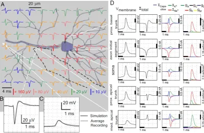
(12) various chemicals [6, 25-30] and different patterning protocols for patterned cell adhesion [8, 31-34].. 1.2.2 Modeling extracellular potentials generated by neural cells Two main types of signals can be identified in an extracellular recording. One is the local field potential (LFP) which has a relatively low frequency content whereas an action potential (AP) has more high frequency content. The extracellular spike recorded from a specific neuron is considered to be repeatable, although this is questionable since the extracellular action potential (EAP) can change, especially during bursts [10, 21]. The magnitude of the recorded EAP depends on the morphology of the cell, the transmembrane currents, the sealing resistance of the cell-electrode interface and the orientation and distance from the electrode to the source [35-36]. The transmembrane currents are affected by the type and number of ion channels, which depend on the type and size of the cell [4]. Gold et al. [35] have investigated by experimental and modeling techniques the effects of the above considerations on the extracellularly recorded waveform. They found that the electrode position had a significant impact on the recorded shape. More specifically, when the electrode position was close to the cell’s body then the EAP was mainly biphasic with one negative peak followed by a slower positive rebound, without any initial positive peak (Figure 6). In contrast, close to the apical trunk the initial positive peak becomes more pronounced. Furthermore, the axon’s initial segment has a slightly lower depolarization threshold and is activated slightly (0.5 ms) before the soma. Therefore, an electrode in this position would record a depolarization at about 0.5 ms before the start of the three-phase EAP. Myelinated areas of axons and nodes of Ranvier do not contribute to the recorded EAP. Finally, the distance of the electrode position was found to affect the width of the negative peaks. The larger the distance the more EAPs may sum up, increasing the total width of the EAP.. 7.

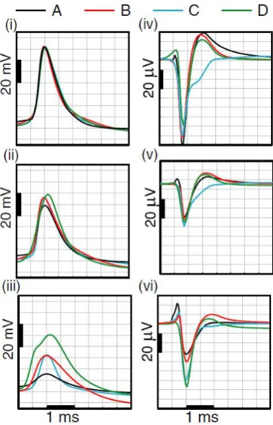
(13) Figure 6. A: EAPs in the transverse section containing the tip of electrode track (dotted line), about 5 μm caudal to the soma and apical trunk (the z-axis is the axis perpendicular to the plane of the section). Close to the soma, there is no initial, positive peak in the EAP. At locations along the apical trunk, the initial peak becomes pronounced. B: comparison of extracellular recording (strongest channel of the tetrode) and simulation at the estimated electrode position. There is only a slight hint of a positive deflection before the negative Na-dominant phase of the waveform. C: comparison of intracellular recording and the simulation in the apical trunk approximately 120 μm from the soma. D: further simulation details. In the soma (middle row) the positive capacitive current, proportional to the change in membrane potential, coincides with the larger Na current (3rd column) because the membrane potential change is driven by local Na current. In dendritic compartments (4th and 5th rows) the membrane depolarization is initially driven by Na current from the soma, until local Na currents are activated and the action potential regenerates. In the brief time before the local Na currents activate, the positive capacitive current is the dominant membrane current and a capacitive-dominant phase is visible in the net current (2nd column). Consequently, the EAP has a more pronounced capacitive phase close to the apical trunk. Also shown, the Na current starts to enter the axon initial segment (2nd row) in a gradual way, driven by the action potential in the first node of Ranvier (not shown) and before the start of the main action potential at the soma. This results in a slightly negative slope in the extracellular potential before the start of the main EAP. Taken from [35].. The shape of an EAP does not depend only on the position of the electrode. The morphology of a neuron affects the waveshape also. The distribution of active ionic conductances can affect its form [37]. In general, the Na+ conductance is responsible for the large negative peak observed in an EAP and its inactivation together with activation of the K+ conductance give rise to the repolarization phase of the EAP. Not all recorded wave shapes look like the EAPs in Figure 4 and Figure 6. Figure 1 is only indicative of Na+ and K+ conductances. Conductances found in cells include fast inactivating Na+, A type K+ (proximal and distal varieties), C type voltage and Ca2+ dependent K+ conductance, D type K+ conductance and K type K+ conductance among others [37]. In order to analyze how the EAP waveform depends on the density of active ionic conductances, Gold et al. [37] created a model and performed four different simulations, each with different ionic conductance distributions. The models had nearly identical intracellular action potentials (IAP) so that only the influence of different ionic conductances was investigated. Their results indicate that. 8.

(14) the shape of a recorded EAP depends not only on the position of the electrode but also on the conductance density distribution (Figure 7), since in different regions of the neuron different types of conductances can be found.. Figure 7. Comparison of Intra and Extracellular Action Potentials for four conductance density models. Left column: IAP at soma (i), and on the apical trunk at 100 (ii) and 200um (iii). The IAPs at the soma are indistinguishable. Right Column: EAP measurements near the soma (iv), near the apical trunk 50 μm (v) and near + the apical trunk 100 μm (vi) from the soma. In model C, repolarization depends on the A type K conductance which inactivates much faster then other types of conductances and makes the repolarization phase of the EAP at the soma somewhat “curvy”. Taken from [37].. 1.2.3 Preparation of networks on traditional MEAs The procedure of plating a culture on conventional MEAs includes decapitation of new-born rats which are then plated on top of a glass substrate integrated with electrodes of diameter 10 – 30 μm. Cells taken from older animals usually have lower probabilities of survival [3]. Only the soma of each neuron is being plated on the MEA. Axons and dendrites do not exist at that time but they form later, during development of the network in vitro. The distribution of cell types in vitro has been found to be the same as that in vivo for networks of cortical neurons. Approximately 10% is inhibitory and the rest excitatory [38-39]. In the preparation of cortical networks cell purification procedures are not common and the culture contains all the types of cells present in the cortex, including glial cells [3].. 9.

(15) The cells are plated within a chamber of diameter 20 mm [3]. A liquid medium (Rominj’s serum - free medium) necessary for growth is added containing a balanced solution of ions and other substances [40]. The network can then grow, form connections, and after approximately 7 days in vitro (D.I.V.) shows spontaneous activity. It may be evident that the number of cells (or cell density) might affect the development of the network [41]. Obviously, if there are just a couple of neurons they may not survive long enough to form a network. Useless cells tend to die due to lack of growth factors secreted by their postsynaptic partners [2]. However, with a higher number of cells in a MEA the recorded patterns are much more complicated to analyze and therefore a balance should be found between density and survival. Furthermore, the lower the density of the culture, the lower the probability that one electrode in a conventional MEA will be close enough to record its activity. A typical culture with 150000 cells in such a MEA can survive for months [3, 42]. In the literature many different densities have been investigated, from 100 cells/mm2 to 2000 cells/mm2 [3, 42-46]. Jun et al. [44] assessed densities as low as 100 cells/mm2 for finding the minimum neuron density and their results indicate that for spontaneous activity a minimum of 200 cells/mm2 is needed and for bursts the number goes to 400 cells/mm2. Ito et al. [47] have recently investigated the minimum cell density necessary for burst generation. Five different plating densities were investigated (2000, 1000, 500, 250 and 100 cells/mm2) and it was found that the minimum density for burst generation is 250-500 cells/mm2. Furthermore, cell densities of surviving neurons at 30 DIV were much lower than initial cell densities ( 1 DIV ).. 1.2.4 Network development Every ex-vivo developing cortical network shows spontaneous activity, starting from the end of first week [10, 12], which changes according to the age of the network [3, 10-14]. Two distinct classes of firing can be distinguished, tonic activity and bursts. Tonic activity is seemingly uncorrelated activity while bursts are composed of synchronous firing and an increase in the recorded activity. Chiappalone et al. [10] and van Pelt et al. [12] have both investigated the spontaneous activity patterns during in vitro development. Their results indicate that the network goes through developmental changes which also affect the recorded activity. Both report on significant developmental changes between the second and third week in vitro. At first, the network forms a surplus of network connections which at a certain point (2-3 weeks in vitro) will be reduced. At the end of the third week in vitro (WIV) dendritic spine and shaft synapses have attained their maximum. 10.

(16) numbers [48-49]. During the 4th WIV dendritic spine synapses are pruned, but not shaft synapses [12]. At a very early stage, the networks exhibit mostly uncorrelated firing, without signs of organization and the activity of the network, measured by the mean firing rate, is close to zero. From that point, the network’s activity increases, reaching a peak at approximately the end of the third week and starts decreasing (Figure 8A). A similar pattern is observed for the bursting activity (Figure 8B). Furthermore, the burst duration was also found to be dependent on the age of the culture with young cultures exhibiting fewer bursts but of higher duration than mature cultures (Figure 9). As stated by van Pelt et al. [12]: “It is remarkable that the time point of maximal synapse number appears to coincide with the time at which network bursts attain their longest duration, and that the period of strong reduction in synapse number coincides with the period in which network bursts develop extremely short rising phases”.. Figure 8. Changes in the spontaneous mean firing rate (MFR, spikes/s) and mean bursting rate (MBR,. burst/min) during the five ages of the monitored cortical networks. (A) MFR averaged over all the recording electrodes from 10 cortical cultures at the considered developmental stages. (B) MBR averaged over all the bursting channels (i.e., channels presenting at least 2 bursts in a recording trial of 5 min) from 10 cortical cultures at the considered developmental stages. All the data are presented as mean + SEM. Reproduced from [10].. 11.

(17) Figure 9. Burst duration and burst number at different ages. All the experiments are reported in the graph. Each point represents a bursting channel producing a certain number of bursts (horizontal axis) whose mean duration can be read on the vertical axis. It is worth noting the change of the network state between the second (14 DIV) and the third (21 DIV) week. The subsequent ages (28 DIV and 35 DIV) tend to group in a region that is the intersection between the two clusters at 14 and 21 DIV, possibly indicating a more stable condition. Reproduced from [10].. Wagenaar [50] investigated the development of high and low density cultures. For the MFR development results were similar to that of Chippalone et al. [10] but sparse cultures showed a more delayed development. A procedure was also created to analyze bursting. The burstiness index (BI) as defined by Wagennar takes values of 0 (no bursts) up to 1. A value of 1 means that all spikes occurred in bursts. He found that although the MFR reaches a plateau and then decreases, the BI continues to increase even after the MFR decreases. 1.2.5 On high-resolution MEAs The main problem of conventional MEAs is that they do not allow a one to one investigation of neural activity. The recorded activity is from a very small percentage of the population. Therefore, a detailed analysis in the investigation of pre-synaptic and post-synaptic patterns is not feasible. When analyzing plasticity between two spike trains, the pathways could be poly-synaptic and in the transition from mono to poly-synaptic pathways the properties of plasticity might be significantly altered. The low number of electrodes together with the high-density of cells necessary for recording can only yield insight in the overall activity of the network and not in relations between poly-synaptically connected cells.. 12.

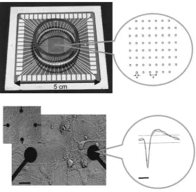
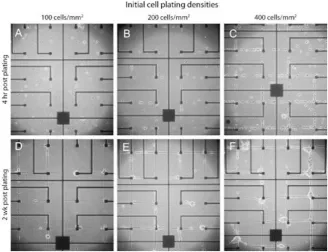
(18) One possible solution could be the patterning of the array with neurotrophic factors in order to direct neuron cell bodies to electrodes [8, 31-34, 44-45]. This way, large regions of neurotrophic factors can attract cell bodies, whereas narrow lines can direct process growth [51]. However, it was found [44] that with increasing cell density the cells tend to grow processes independent of the patterned surface and with lower density cultures the network is not active (Figure 10). Another approach is the development of high-density MEAs, consisting of thousands of electrodes with electrode densities similar to densities of the culture. A 1 to 1 correspondence between electrodes and cells might then be achieved. Berdondini, Imfeld et al. [52-53] have presented a high resolution system for data acquisition of electrophysiological recordings based on an active pixel sensor array (Figure 11). Main components of the platform are an integrated microelectrode array, low noise amplifiers and high-speed random addressing logic. The device’s concept is based on image/video data capture methods implemented on hardware. 64 x 64 electrodes arranged as an array of pixel elements constitute the MEA. Electrode sizes are 20 μm x 20 μm and the electrode separation is 20 μm while the total active array is 2.56 mm x 2.56 mm. The resulting electrode density is then 625 electrodes/mm2 [53]. Typical noise levels are quite high (11 μVRMS) but signal to noise ratios of 5-10 have been accomplished [52]. Other drawbacks of the system include limited usage of each chip (4-5 experiments, 30 DIV for each experiment) and an increase in the number of non working electrodes after intensive use. Furthermore, no in-pixel stimulation capabilities exist, but rather only through dedicated electrodes. Another approach from the same group includes locally dense microelectrode arrays (Figure 12) [54] in which 60 microelectrodes are arranged in four areas separated by 1.1 mm. Each area features 15 microelectrodes with 10 μm interelectrode spacing. Electrode diameters were 30 and 22 μm. Finally, the ADC resolution was 12 bits and sampling frequencies ranged from 10 to 50 kHz/channel. Recordings showed that 60% of the electrodes pick up signal from one neuron. The other electrodes would pick up signals from two neurons with one being the dominant (90% of the events), allowing a very accurate mapping of electrodes to cells. Furthermore, with increasing sampling rate propagation of the spikes could be identified. Typical noise levels were 8.2 μV (22 μm electrode diameter) or 6.5 μv (30 μm electrode diameter). We must note here, that although the larger diameter electrode has lower noise levels, it is more prone to picking up signals from more than one source. The main disadvantage of this system is the limited active area. As illustrated in Figure 12 the area covered by electrodes is small compared to the area of the ΜΕΑ.. 13.

(19) Figure 10. Phase micrographs of live neurons growing as networks on patterned poly-l-lysine MEAs. 2. Cells were plated at initial seeding densities of 100, 200, and 400 cells/mm . Images are presented illustrating cultures at 4 h and 2 weeks after plating. The big black box is the ground of the system. Small, rectangular boxes represent places for cell bodies while the black lines aim in directing process growth. Notice that with increasing plating density neurons tend to escape from the patterning scheme. Reproduced from [44].. 14.

(20) Figure 11. Overview of the high resolution electrophysiological platform. The system is composed of. three hardware levels, i.e. the CMOS–MEA chip, the interface board and a work station equipped with a frame grabber for capturing and storing the video stream. Taken from [52].. Figure 12. View of a locally dense microelectrode array. Reproduced from [54].. 1.3 The ETH 11000 electrode, CMOS system Typical MEA system designs contain the electrode array separated from the signal conditioning electronics [55-57]. Each electrode requires a connection to the external electronics, limiting the array size. Furthermore, the signal should be conditioned as close as possible to its source to prevent noisy data. The requirements of high signal-to-noise ratio and a large number of electrodes seem difficult to be accomplished together. This stems from the fact that for high density MEAs the available space for each electrode and its accompanying electronics is limited. However, the smaller the size of electronics the higher the thermal noise.. 15.

(21) The end result is that when using high-density MEAs noise levels are quite high, making difficult the extraction of electrophysiological signals [58]. The majority of commercial MEAS currently in production are termed passive. This means that no active elements (amplifiers, mutliplexers) are integrated on chip. Each electrode requires an external connection to filters and amplifiers. This approach poses a limit on the maximum number of electrodes on the substrate, since each electrode requires a connection to external electronic circuitry. Furthermore, the signal is not amplified close to its source. In the pathway from the electrode to the amplifier, cross-talk may occur which hampers the signal to noise ratio (SNR). The Bio-engineering laboratory of ETH (Swiss Federal Institue of Technology, Zurich), headed by Prof. Andreas Hierlemann conducts research on developing microelectronics-based tools for solving problems in biology. Recently they have developed a switch-matrix based high-density microelectrode array in CMOS technology suitable for physiological recordings [59]. The device has been sent to several collaborating groups for debugging, including:    . Laboratory for systems biology, RIKEN, Japan University of Freiburg, IMTEK, Germany. University of Bern, Switzerland. Twente university, the Netherlands.. In the BSS group, people working on the theme of Neurotechnology, lead by prof. Wim Rutten have therefore access to the high-density chips for physiological recordings. The system consists of a microelectrode array of 11011 electrodes, 126 of which can be arbitrarily selected using reconfigurable electrode-readout-channel mapping. The front-end circuitry is then placed outside the array itself, allowing sufficient space for low-noise circuitry and providing high-density of electrodes. Electrode diameter is 7 μm, electrode pitch 18 μm and electrodes have also the ability of stimulation. Noise levels are low (3.9 μVRMS, 1 Hz to 100 kHz, bare Ptelectrodes ) and electrode density is 3150 electrodes/mm2. The increased electrode density allows plating of low density cultures (cells/mm2) while the low noise levels allow recording of low-amplitude spikes. Two main advantages of using integrated circuit or CMOS technology include connectivity and signal quality [4, 59]. Using on-chip multiplexing architectures allows the use of a large number of electrodes. When the signal is conditioned close to the electrode the SNR increases, allowing better observation of weak physiological signals such as extracellular spikes. A disadvantage of such IC chips is that silicon is not transparent to light, which makes the observation of cells through a light microscope impossible. Furthermore, the. 16.

(22) chip must be protected from the bath medium used to culture the cells and the culture must be protected from toxic substances used in the chip. For example, CMOS metal aluminum dissolves in saline solution [4]. However, deposition of platinum makes the electrodes biocompatible.. 1.4 Formulation of research questions Cultured neuronal networks on MEAs provide a useful platform to study cognitive processes like learning and memory. Essential in such research is the ability to estimate network connectivity. Most tools to estimate functional connectivity are based on the analysis of activity patterns, and there are indications that such estimated functional connectivity provides information about physiologic, synaptic connections. However, a thorough validation is hampered by the fact that it is not possible to visually trace axons on the chip due to the high density of seeded cells. This high density is necessary because at lower cell densities the probability that one of the 60 electrodes record activity falls significantly. This means that due to the undersampling of the culture’s activity with the 60 electrodes, the culture may be active but no electrode would be close to a cell to record its activity. Recently, we obtained the switch-matrix based, high-density microelectrode array device designed by ETH, Zurich, for use in our group [59]. The high density of the electrodes allows us to record activity even from low-density cultures, with the appropriate electrode selection. So, a first challenge is the development of an efficient way to select the 126 electrodes to record from. Then, activity analysis and the culture’s development will be investigated. To sum up, basic research questions include:     . How can we efficiently find the most suitable electrodes to record from? How stable is the recorded activity from this set of electrodes? What are the differences in spontaneous firing patterns in high and low density cultures? What is the minimum network size/density that we can record activity from? How representative is a set of electrodes?. 17.

(23) 2. Methods and materials 2.1 Hardware 2.1.1 System Description In this section the system’s electronic components will be described. A block diagram of the whole system is shown in Figure 13. The chips are plugged in the chip-support board, called the Neurolizer, which provides all necessary clock and digital control signals together with the required analog references to the chips. Data are serialized on the board and sent through a serial connection (LVDS protocol) to an FPGA board. The FPGA runs Linux operating system, performs CRC checks of the chips, separates data streams from different chips and finally, transmits the data to the PC used for data analysis, visualization and storage. The PC runs a server application, named the server, which can be accessed from several clients requesting data or sending commands. The server contains emulators of the chips. When a command is sent to a chip the same command is applied on the emulator of the appropriate chip. The client can then request from the server information about the chip routing, gain and filter settings etc. through a TCP/IP connection. Figure 14 shows the system’s data flow. The FPGA board sends the received data first to the server. The server contains a buffer of 25seconds. This value can be changed in the defines.h file located at: cmosmea_external/ntk_tools/trunk/resources/defines.h The client(s) can then request data from the server, specifying the amount of data (10, 20, 100 ms) and the interval between successive requests. If there are not enough data, the client has to wait before receiving the data package. If the client reads data too slow, the buffer will fill and the client will lose data. The color of the buffer will then change to red. More than two clients can request data from the same plug, there is no “interference” between the two. Finally, the client can request data in two modes, stream or live. In the stream mode, the server keeps track of the position of the latest data and sends the next package according to that index. In the live mode the server always sends the newest data. When a command is sent, if it is successfully executed it will then proceed to the server’s emulator. It is also important to note that when a command is sent there is no accurate timing; it depends on the computer load, speed and SNR of the transmission pathways (Ethernet) among other conditions.. 18.

(24) Figure 13. Block diagram of the system. A photograph of the support board with plugged in chips is shown on the left. Taken from [59].. Figure 14. System data flow. Commands follow a different path than data. Notice that there is no accurate timing in a command execution. Data can be saved directly from the server (which can also attach commands in the recorded file) or by the client (e.g. Labview, which only see the data and not the commands). The client can select which chip to read from through the server or the client (which communicates with the server). Taken from [60].. 2.1.2 Chip description The chip is mounted on a custom-made printed circuit board (PCB) with an electroplated nickel/gold edge-connector. A glass ring is glued on the PCB and a water-resistant epoxy is used to encapsulate the bond wires and pads. The packaged device is shown in Figure 15 and a micrograph of it in Figure 16. The 126 channels and the associated signal amplification and stimulation circuitry are outside the reconfigurable electrode array.. 19.

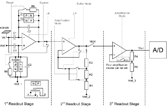
(25) There are three signal conditioning stages on the chip. The first two stages include signal amplification and filtering, whereas the third only includes amplification. The first stage includes a high pass filter, a low pass filter and an amplification of 30 dB. The second stage includes a low pass filter, an additional gain of 0, 20, 30 dB and a DC-Offset compensation scheme. Chip settings (gain, cut-off frequencies) are all set to the same values for all channels. After the second stage, eight channels are multiplexed and amplified at 0, 6, 14 or 20 dB and finally, digitized with an 8-bit ADC. The recording controller then transfers the data off-chip. The command decoder is responsible for commands of array configuration, gain and filter settings. Finally, 2 10-bit DACs provide stimulation capabilities. Figure 18 shows the schematic of the three signal conditioning stages. The gain of the first stage is defined by the capacitance ratio C1/C2 and is 30 dB. The LPF cut-off frequency can be selected to 15 or 50 kHz. The default HPF cut – off is below 1 Hz. A switch provides a complete bypass of the first stage to test features in DC. The second amplification stage is a non inverting amplifier implemented as a two stage Miller compensated opamp. Switching between different resistors R1 , R2 , R3, adjusts the gain selection. The LPF cut-off frequency can be adjusted to 5 or 16 kHz. The DC-offset compensation scheme can remove DC signals of up to 55 mV in steps of 5 mV. After the 3d stage data are transferred to the digital part of the chips. The 16 ADCs run at a clock speed of 3.2 MHz and need 10 clock cycles for one 8-bit conversion. One frame of output consists of 160 bytes, 128 of which are used for data and the rest for status information about the device (gain, filter settings etc…). The chip address, the frame counter and the command counter are also inserted. A command is only executed if there are no CRC errors and if the chip address is correct. After a successful command execution the command counter increases. Commands are used to change the amplification factor and adjust DC-Offset compensation.. 20.

(26) Figure 15. Packaged device. Taken from [59].. 2. Figure 16. Micrograph of the fabricated device. The size of the chip is 7.5 x 6.1 mm , the size of the 2 electrode array is 2 x 1.75 mm . Taken from [59].. Figure 17. Block diagram of the chip architecture and the on-chip electronics. Taken from [59].. 21.

(27) Figure 18. Amplification stages of the readout channels with the first stage featuring a low HPF cut-off frequency. Taken from [59].. 2.1.3 Electrode array and configuration The flexibility of the system is provided by an analog switch matrix implemented underneath the microelectrode array. Its general form is shown in Figure 19. Electrodes are connected to channels through vertical and horizontal wires. The reconfigurable switches control the connections of the wires. Each channel can be connected to any electrode but there are some limitations. Firstly, in Figure 19 it is shown that for the electrodes belonging to the same row, the seventh electrode uses the same transfer line (horizontal wire) as the first one. Or to put it differently, every sixth electrode occupies the same transfer line. This has two implications: 1. A maximum number of six consecutive electrodes in a row can be used. 2. When electroden is used, electroden+ k*6 from the same row cannot be used (k = -2, -1… 1, 2…). This poses some limitations in the final array but due to the large number of electrodes they can be overcome. Limitations also apply for the vertical wires.. 22.

(28) According to the designers of the set-up, the largest block of electrodes possible is a 6x17 rectangular configuration.. Figure 19. Illustration of the switch matrix reconfigurable array. The selected electrodes (1-6) are being routed to the output channels (A-F). Taken from [59].. The final configuration is controlled by specialized software (NeuroDishRouter) which solves the routing problem. Another software (BitStreamer) creates the command file that can be sent to change the configuration. Possible configurations are blocks of electrodes, random electrodes or single spots. NeuroDishRouter can also create a sequence of files to scan the whole array.. 2.2 Culture preparation and maintenance Active and healthy cultures are the most basic materials for our experiments. Newborn Wistar rats were decapitated and cortical neurons were obtained and cultured within a circular chamber on the CMOS chip. For high density cultures the seeding concentration was 3 million cells/ml. A drop of 30 μl was then applied on the array chamber, resulting in an initial plating density of 2500 cells/mm2. The culture chamber was filled with 600 μl serum-free medium [40]. Cultures were stored in an incubator, under standard conditions of 37o C, 100% humidity and 5% CO2 in air. In the incubator the cultures’ surrounding air is in contact with the incubator’s environment, allowing the exchange of gases. The cultures are not visually inspected in their various development stages due to the non-transparent nature of silicon. The medium was refreshed three times a week in each culture. Approximately half of the medium is taken out and slightly more is added (because of medium evaporation).. 23.

(29) 2.3 Experimental procedures After a medium change, the cultures were left in the incubator for 3 hours before any experiment took place. Measurements took place inside a dry incubator. Each culture was covered with a film allowing gas but not water exchange to protect it from bacteria and infections. The incubator was dry so that there was no risk for the electronics. However, medium evaporation takes place and it was found that when leaving a culture for 2 days with the lid not properly sealed the entire medium evaporates and the culture dies. 2.3.1 Verifying hardware’s and software’s integrity with physiological saline The first phase of the experiments was to verify the suitability of the hardware and newly-developed software for performing the experiments. The chips were filled with 600 μl of saline and signals were recorded for 50 minutes. In the duration of the experiments, gain, electrode configurations and other settings were changed in order to verify their correct operation. Typical noise levels were also registered. Only connected electrodes were taken into account. Temperature was recorded in order to set the externaly controlled temperature (incubator) to appropriate levels. The maximum temperature of the chips should not exceed 37 °C. The temperature was recorded with two conditions. In the first case, the incubator’s temperature was set to 34.7°C and in the second case to 33°C. A sensor was attached underneath the MEAs to record their temperature for 50 minutes (see appendix for the experimental set-ups). This duration seemed appropriate for the experiments of this project. No long recordings took place so a temperature recording of hours or days was deemed unnecessary. For verifying the integrity of our newly-developed software we used sample data from the University of Kaiserslautern and compared results from our software to the results of the hidens toolkit. Spike shapes and raster plots were produced to get an idea of the signals obtained. 2.3.2 Trial experiments with active and silenced cultures Following verification of the experimental set-up, recordings were made in order to analyze the activity and development of high- density cultures. Recordings were made with a random electrode configuration to assess culture’s properties and electrode activity and stability of the set. The cultures’ activity was then analyzed for different DIV assessing their activity patterns. Data from these experiments were used to analyzed the activity of cultures, the stability of electrodes, the performance of the electrode selection algorithm, spike shapes and burst profiles. As a final step,. 24.

(30) magnesium was added in the medium in order to verify that identified events are actually cell extracellular potentials and not artifacts. Magnesium is known to stop all spontaneous activity of the culture. If the activity recorded in the baseline phase was indeed from spontaneous activity of the network and not artifacts, then the identified activity in the magnesium phases should be minimum. Magnesium sulfate was used with a molecular weight of 95.22 gr. For adding 1mM of magnesium to 600 μl of medium we need 57 μgr of the substance. MgSo was diluted in physiological saline (57 mgr in 1 ml) and then 1 μl of that substance was added to the 600 μl of serum-free medium. The amount added is insignificant compared to the total amount in the culture and should not alter the activity of the network. A baseline recording took place, followed by addition of 1 μl of plain, R12 medium to check for protocol effects (adding 1 μl of a substance, control phase). Then, 1 μl of MgSo was added for the Mg phase. The Mg-filled medium was then washed out twice and replaced by 600 μl of medium for the washout phase. The duration of the recordings was 20 minutes and the first 5 minutes of each phase were ignored because handling of the cultures was shown to affect their activity, mostly in the first 5 minutes [50]. 2.4 Algorithms and techniques 2.4.1 Electrode selection overview The electrode selection algorithm should be able to find a local/global set of electrodes that will allow us to record high quality signals. By quality of the signals we mean low noise levels, large spike amplitude and high enough firing rates. With high density cultures selection of such an electrode set should not be difficult, but with lower densities a more thorough search through the search space should be done. As a first step, a “brute-force” attack was used for this search. This method evaluates all possible sets of solutions to find the best one. Therefore, all electrodes were used in some sample recordings and their suitability was evaluated. This procedure is termed “Scanning algorithm”. 2.4.1.1 Scanning algorithm and electrode evaluation This procedure scans all electrodes of the array in sequential blocks, generated by NeuroDishRouter. The scanning procedure includes the following steps:. 25.

(31)    . Select configuration Send configuration to the server Record with online spike detection algorithm Repeat for all configurations. Each configuration needs 1 minute in total. Specific command files for each configuration were created. After sending the configuration and before spikes are accepted, the DC-Offset compensation scheme is applied. This scheme is already implemented in the Lab view hidens toolkit. Its automatic application after a configuration change was implemented for the needs of this project. Furthermore, noise values need to be re-established, so the first 10 seconds of a new configuration are ignored. This amount of time seemed satisfactory based on our observations. Noise levels need 3-4 seconds to stabilize, so a value of 10 seconds is more than enough. The detailed procedure is explained in the following section. The output file is an events-file containing information about the events. It is then loaded into Matlab which produces the final configuration of the electrodes after their evaluation. Electrodes are evaluated based on certain thresholds:    . The Mean Firing Rate (MFR) should be above a minimum value. The average noise levels should be below a maximum value. The number of points above threshold levels should be above a maximum value. The spike’s amplitude should be above a minimum value.. 2.4.2 Online spike-detection algorithm The online spike-detection algorithm is threshold based. The RMS noise value for each electrode is calculated and when the threshold (5.5 times the noise levels) is passed (negative only) an event is identified and recorded. The threshold value is adjustable. However, three more constraints were added to improve efficiency. 1. Saturated electrodes Each electrode can have DC potential fluctuations, also called drift. The DC offset compensation scheme is applied in the second stage of the amplifiers, so if the first stage is saturated, the DC offset compensation scheme will not solve the problem.. 26.

(32) When an electrode is saturated, the noise is extremely low and because of that, spikes can be wrongly identified when the signal’s value crosses the threshold (which depends on the noise levels). The false positive rate then is extremely high for that electrode. In the Hidens matlab toolbox when such a signal is observed it is ignored. For the purposes of the online spike detection algorithm a constraint was added. If the noise of the electrode is too low, spikes are not identified in that electrode. The electrode should have a minimum noise level. The value of this parameter can be changed in the settings tab of the software and values used were up to 8 μVs. 2. Idle time after a configuration change (DC-Offset) When changing configurations it is important to automatically apply a DCoffset compensation after some time due to the fact that each electrode has a different DC value. This functionality has been implemented in the software and affects the online spike-detection algorithm. When such a compensation is applied, due to the sudden change in the recorded values, spikes would be wrongly identified. Therefore, spikes are ignored after application of the DC offset compensation in the scanning algorithm for 5 seconds. Channels are compensated in parallel. Each configuration change need 5 seconds for all channels, not for each. A boolean control was implemented (when the value of this boolean control is false, spikes are not identified) and for 5 seconds after the configuration change, spikes are ignored to allow sufficient time for the change to take place. 3. Idle time before DC-offset compensation For the electrode selection algorithm, or when manually changing configurations, one recording is made in which all electrodes are used by using sequence recordings. When a configuration is changed, data should be ignored for some time after the change, allowing the noise levels to stabilize for the given new configuration, like in constraint 2. Otherwise, spikes will be wrongly identified during the transition from one configuration to the other. A boolean control was implemented (when the value of this Boolean control is false, spikes are not identified) and for 5 seconds after the configuration change, spikes are ignored to allow sufficient time for the noise levels to be estimated. After these 5 seconds, the automatic DC-Offset compensation scheme takes place so the total idle duration is 10 seconds. The output of the detection algorithm is a file containing information regarding:. 27.

(33)    . Time of the event Electrode (not channel) recording the event Waveform (6 msecs, in μVs) Noise Levels during the event. 2.5 Data analysis For data analysis we used mean firing rates (MFR), mean bursting rates (MBR), raster plots and other graphs illustrating the activity development of the cultures. The MFR and MBR are defined as the number of events and bursts per minute respectively. A burst is defined as a collective, sudden increase in the activity of the network. All spike trains were divided into time segments of 2.5 minutes. Calculations for the firing rates at a specific DIV include the average and std of these time segments. This approach has been followed for a single reason. The activity of the network might not be stationary; By averaging (using appropriate time-segments) a better indication of the firing rates is obtained. Furthermore, the MFR (and MBR accordingly) might change and by re-calculating the burst threshold according to the MFR in each time segment the accuracy of the burst identification (explained later in this section) is improved. Raster plots indicate the firing patterns of the network. One can visually discriminate if the culture exhibits bursts or not. A disadvantage of this method is that one can only observe a finite amount of time. Usually this interval is approximately 1-5 minutes. With higher intervals details on the exact timing of spikes are lost. Together with raster plots the binned number of events is illustrated for easy visualization of the activity pattern. The bin size was set to 30 ms, a value small enough to yield detailed description of the activity fluctuation and an easy to visualize plot. Individual electrode activity was analyzed for all cultures. The MFR of individual electrodes was calculated and data sets were later interpolated (cubic spline interpolation) and averaged to give one average for all cultures and electrodes. The stability of the electrode set can be evaluated by observing the number of electrodes that appear or disappear from one experiment to the next. As a final step we calculated the number of active electrodes in each experiment for all cultures. An electrode was considered active if it showed more than two spikes per minute and the number of active electrodes is plotted for each culture and DIV. Finally, during the cultures’ development the properties of spike shapes and burst profiles are shown. The spike shapes were clustered according to two properties: . Peak to peak amplitude (Vpp). 28.

(34) . Peak balance (PB). The peak balance is an indication of the spike shape and it allows discrimination between different spike shapes. It is the difference of the areas of the two positive phases of the spikes, before and after the negative phase respectively. Almost all burst shapes are shown in order to see their amplitude, duration and general shape. The number of events per bin is also counted and bursts are identified by an automatic procedure, previously used in [61]. The threshold for burst detection has been set to 9.5 times the average MFR of the time segment analyzed. This value was carefully selected after evaluation, see appendix for the details. When a burst was found its profile was calculated for 0.5 seconds before and 0.5 seconds after its center (center defined as the peak of the amplitude). Threshold crossings were treated in order of size and overlap between profiles was prevented by setting all the bins around the detected burst to 0 (duration 2 seconds) after the calculation of the burst profile. The value of 0.5 seconds proved adequate to capture the burst profiles and the duration of 2 seconds was deemed low enough so as not to erase nearby bursts since inter-burst intervals are in the order of 10ths of seconds [10]. After obtaining the burst’s profile we calculated the number of events in it. The width of the burst was calculated as the distance between the 10% points before and after its peak. The number of events in this segment was then counted. The number of events in bursts divided by the total number of events in each segment give the Burst/dispersed ratio. This is an indication of how many spikes are in and out of bursts. A value of 100 % means that all spikes occurred in bursts. Different sets of electrode configurations were compared in order to analyze the effects of different configurations on the activity recorded. Recordings with different configurations include comparison among three random and block configurations. Finally, a scan of the whole array was performed to find suitable recording electrodes. To answer the question of which one is the limiting factor in choosing an appropriate set of electrodes, colormaps of active electrodes were produced for their MFR, average spike amplitude and average noise levels. Different sets of electrode configurations were then compared to the optimum one. This optimum set is a subset of the suitable electrodes found. More specifically, a random configuration, a block configuration, a conventional configuration (rectangular array of electrodes) and the best configuration are compared to each other. The conventional configuration is one similar, but obviously not the same as in conventional MEAs, due to electrode routing limitations, size and pitch.. 29.

(35) 3. Results 3.1 Verification of experimental set-up 3.1.1 Saline experiments As a first part of the project, the incubator’s appropriate temperature was investigated and noise levels were established. The maximum temperature for a culture is defined around 37°C. From the two experiments conducted (with incubator settings for the external temperature: 34.7°C and 33°C ) it can be seen that when the external temperature is set to 33°C, the temperature of the culture stays below 37°C for almost one hour after starting the experiment (Figure 20). Therefore, in all subsequent experiments the external temperature used was 33°C. Figure 21 shows noise levels for the three experiments during which the external temperature was set to 33°C. Saline experiments conducted on three chips. Noise values from all channels were recorded. Three basic categories can be distinguished, extremely low noise channels (saturated channels, less than 3 μVRMS) and two other separated distributions. The left one is composed of unconnected channels (6 – 9 μVRMS) and the second from connected channels (10 – 16 μVRMS).. Figure 20. Temperature was recorded 0, 10, 20, 30 and 50 minutes after starting the operation of the device (server receiving data). See appendix for screenshots of the experimental set-ups.. 30.

(36) Figure 21. RMS Noise levels during saline experiments. Saline experiments conducted on three chips. Noise values from all channels were recorded. Three basic categories can be distinguished, extremely low noise channels (saturated channels, less than 3 μVRMS) and two other separated distributions. The left one is composed of unconnected channels (6 – 9 μVRMS) and the second from connected channels 10 – 16 μVRMS).. 3.1.2 First spike shapes and ISI Histograms First spike shapes observed with active cultures are shown in Figure 22a. Spike shapes are clearly distinguishable from background noise. All histograms of each culture (all data used for analysis) were summed up and the results are presented in Figure 22b. It is obvious that there almost 0 spikes with ISI of less than 1 msec. furthermore, a peak is observed in all cultures at 40 – 50 ms. a. b. Figure 22. (a) Illustration of recorded spike shapes. (b) Interspike intervals for all experiments and all cultures. All I.S.I. were summed up, producing these final figures. The first bin, with bin center of 0.5 includes values of 0 to 1 msec.. 31.

(37) 3.2 Dynamics in developing high density networks 3.2.1 Basic electrode configuration and raster plots The random electrode configuration used for the experiments is illustrated in Figure 23. Raster plots of the three cultures showed transitions among different patterns of activity as the culture matures. Raster plots of the development of culture 599 are illustrated in Figure 24 (10-19 DIV) and Figure 25. (21 – 28 DIV). Below each raster plot the number of events in each bin is shown (bin width = 30 ms). Bursts are shown in these plots with an asterisk situated on the center of each burst. Both uncorrelated firing and bursts were observed during the culture’s development. More specifically, an increased number of bursts was observed in 10 DIV (Figure 24a), and in 25 and 28 DIV (Figure 25b-c). Small and large fluctuations of the spontaneous activity are observed even when the bursting frequency is low (Figure 25a) with the strongest fluctuations identified as bursts. A clear transition can be seen from 10 to 11 DIV (Figure 24a,b) from bursting (extremely low or high number of events per bin) at 10 DIV to a more stable firing pattern at 11 DIV. Raster plots for the other cultures can be found in the appendix.. Figure 23. Random electrode configuration used for activity analysis of the three cultures. This. configuration was used in all experiments and all cultures, unless written otherwise. The size of the 2 array is 2.0 x 1.75 mm .. 32.

(38) a. b. c. Figure 24. Raster plots of culture 599 at an early stage of development (10 – 19 DIV,a-c). On the top, a raster plot of 5 minutes is shown. The bottom plot indicates the number of events in each bin (bin size is 30ms). Spike trains were divided in segments of 2.5 minutes. For each segment, the bursting threshold was set to 9.5 times the mean firing rate for the specific segment.. 33.

(39) a. b. c. Figure 25. Raster plots of culture 599 at a mature stage of development (21 – 28 DIV,a-c). On the top, a raster plot of 5 minutes is shown. The bottom plot indicates the number of events in each bin (bin size is 30ms). Spike trains were divided in segments of 2.5 minutes. For each segment, the bursting threshold was set to 9.5 times the mean firing rate for the specific segment.. 34.

(40) Zoomed plots displaying in detail the uncorrelated firing and bursts are shown in Figure 26. Activity preceding bursts could be either zero (figure 26b) or non-zero (Figure 26a). During uncorrelated firing, fluctuations in the activity have been observed (Figure 26c). a. b. c. Figure 26. Raster plots of different cultures illustrating the uncorrelated firing (c) and the appearance of synchronized firing (a,b). In culture 599 (a) the synchronized firing (burst) is preceded by some activity. On the other hand, bursts of culture 512 (b) are preceded and followed by absence of activity. On the top, a raster plot is shown. The bottom plot indicates the number of events in each bin (bin size is 30ms). Spike trains were divided in segments of 2.5 minutes. For each segment, the bursting threshold was set to 9.5 times the mean firing rate for the specific segment.. 35.

(41) 3.2.2 Firing rates and active electrodes Analysis of firing and burst rates (Figure 27) agrees with the raster plots. During the first stages of development all cultures exhibit low mean firing rates (MFR, figure 27 first row) and low, but not zero mean bursting rates (Figure 27, second row), with the exception of culture 599 which initially (10 DIV) showed increased burst frequency. MFR reached a plateau at 21-26 DIV depending on the culture and declined afterwards. The number of spikes per minute for cultures 512 and 599 at 11 DIV was higher than 1000. MBR increased substantially in the later stages of development, when the MFR showed a decrease. Accordingly, the percentage of events in bursts occupied a large fraction of the total events reaching values of more than 70% (culture 512, 26 DIV).. Figure 27. Firing rates for all three cultures analyzed. First row shows the mean firing rates (spikes/minute), the second row shows the mean burst rate (bursts/minute) while the third row shows the burst/dispersed ratio. This ratio is the ratio of the number of events in bursts divided by the total number of events. Spike trains were divided in segments of 2.5 minutes and averaged to produce the final value. Errorbars represent the std of these averages. For each segment, the bursting threshold was set to 9.5 times the mean firing rate for the specific segment.. 36.

(42) The MFR of individual electrodes fluctuates much more than that of the whole network. Electrodes with the highest activity showed MFR patterns similar to that of the culture’s MFR (e.g. Figure 28a). Less active electrodes showed more stochastic transitions between active (with low MFR) and inactive phases. Plots for all individual electrodes can be found in the appendix. Figure 28b shows the normalized, averaged MFR of individual electrodes and it is evident that they follow that of the whole network, although with a very large standard deviation. The number of active electrodes (Figure 28c) also corresponds to the culture’s MFR. Depending on the culture, after 20 – 25 DIV the number of active electrodes decreases. Out of the 126 electrodes used in the random configuration, a maximum of about 25 electrodes showed activity at the same day for culture 529. Furthermore, in different stages of development, different electrodes show activity as is illustrated from the high number of electrodes becoming active or inactive from one experiment to the next (Figure 28d). Only a few electrodes become active after 20 DIV.. 3.2.3 Burst profiles Burst profiles as identified by the burst-detection algorithm reveal a change in the burst profiles. Figure 29 shows the burst profiles for all cultures at various, selected, DIV. Culture 529 showed fewer bursts than the other two cultures and only at 28 DIV, so one burst profile is shown for this culture. At a young age, bursts are symmetric, while at a later age, 26 DIV and older, burst profiles, together with burst frequency, change dramatically. Bursts have a very fast rising phase (e.g. around 100 ms for culture 529), with the falling phase being much slower (e.g. around 300 ms for culture 529). Profiles of cultures 512 and 599 at 26 and 28 DIV are similar to that of culture’s 529 at 28 DIV. All shapes, especially the ones in the later stages of development are reproducible. However, in the earlier stages of development (10 – 11 DIV) the burst’s amplitude fluctuates more than that in the later stages of development (26 – 28 DIV).. 37.

(43) a. b. c. d. Figure 28. Electrode analysis. A) MFR for individual electrodes. B) The top plot shows the normalized, averaged MFR of individual electrodes and the bottom plot shows the same results, interpolated. Data from each electrode were normalized to the average of the first two points to produce the normalized data which were then averaged to give one data-series for each culture. C) Development of the number of active electrodes in each experiment (interpolated). D) number of electrodes becoming active or inactive from one experiment to the next.. 38.

(44) a. b. c. Figure 29. Smoothed burst profiles as identified by our burst-detection algorithm for all cultures. Burst profiles, especially in the later stage of development are reproducible. Bursts were identified using a threshold based algorithm, 9.5 times the MFR of each time-segment (spikes/bin).. 39.

(45) 3.2.4 Spike shape clustering The properties of spike shapes for culture 512 (Figure 30a) show a very clear transition. The peak to peak amplitude increases, whereas the peak balance decreases. This means that the second phase becomes more pronounced compared to the first one. The other two cultures have more dispersed properties but culture 529 at 11 DIV (Figure 30b) mostly exhibits spikes of negative balance which also indicates that the second positive phase is much higher than the first one. Four spike shape categories were generally observed and up to 20000 spikes from each experiment were then classified to one of these categories. Class 1 is monophasic, class 2 biphasic with a large first positive phase, class 3 biphasic with a large second positive phase and class 4 triphasic. Figure 31 shows representative examples from each culture (a-c) as well as the percentage of each spike shape. Monophasic spikes occupy less than 50% with the lowest percentage (23%) in culture 512. On the contrary, triphasic spikes reached values of up to 33% in culture 599. a. b. c. Figure 30. Spike shape clustering for culture 512 (a), 529 (b) and 599 (c). The peak to peak value of the spike and the peak balance were used. The peak balance is the difference of the areas of the two identified positive peaks (before and after the negative phase), if any.. 40.

(46) a. b. c. d. Figure 31. Spike shape clustering for culture 512 (a), 529 (b) and 599 (c). Four different classes were identified in all experiments and representative examples are shown. The percentage of each class for each culture is depicted in (d) together with the total number of spikes in the dataset. From each experiment, a maximum of 20000 spikes were taken (where available).. 41.

No results found