Floating ratemortgages: why do they prepay?

October 2010 1 Supervised by:

Dr. R.A.M.G. Joosten - University of Twente Dr. B. Roorda - University of Twente MSc. J.S. Holtman - ING CMRM

Floating-rate

mortgages:

Why do they

prepay?

October 7

2010

Master Thesis C.T.J. Hamstra,

University of Twente, Industrial Engineering & Management. Corporate Market Risk Management, ING.

A Logit model

for prepayment

drivers

They have a floating- rate mortgage…

October 2010 3

Preface

Two years ago I made the decision to advance from a Bachelor at Saxion Universities of Applied

Sciences to a Master at the University of Twente, because I felt an academic Master would give me

valuable skills and insights for future work as an Industrial Engineer.

The first weeks were tough, getting used to a new system and level of education and having to attend

lectures in 4 different classes to be able to follow the Pre-Master as well as the Master curriculum.

Fortunately, the curriculum of Financial Engineering & Management fit my interests in finance perfectly

and, together with a talk with Track coordinator B. Roorda, inspired me to work even harder to finish

the Master. I would like to thank Mr. Roorda for this. In March this year, the final hurdle remained,

which I knew was going to be the toughest, the Master thesis…

This research was conducted for the department Corporate Market Risk Management - Retail

Netherlands (CMRM Retail NL) of ING and in the context of a master thesis assignment for the studies

Industrial Engineering & Management of the University of Twente.

Mrs. J.C.M. van de Rijt, manager of the department CMRM-Retail NL, formulated the research topic

and it was supervised by her and Mr. J.S. Holtman from ING and Mr. R.A.M.G. Joosten and Mr. B.

Roorda from the University of Twente. I would like to thank all of them for their guidance, and in

particular Mr. Holtman for his patience and the pleasant day-to-day collaboration. I thank Mrs. Van de

Rijt for adhering to my request for a more scientific research topic than the one initially planned.

Moveover, I would like to thank Mr. Joosten and Mr. Roorda for their critical assessment of the thesis

and the helpful suggestions they gave.

I am grateful for the help throughout the project of my direct colleagues and in particular Msr. C.

Lubbers-Benning who provided me with insight into the statistical model applied and Mr. R.

Stakenburg and R. Fanciully for data collection and statistical analysis respectively, which has been

essential in getting the results.

My internship, research, and the development of a mortgage hedge-tool have given me insight into the

application of Market Risk management theories in practice, and I have had a more than pleasant time

October 2010 4

Floating-rate mortgages: Why would they prepay?

Preface ... 3

Summary ... 6

1. Introduction ... 8

1.1. Market developments ... 8

1.2. Current situation ... 8

1.3. Problem analysis ... 10

2. Research design ... 14

2.1. Scope ... 14

2.3. Prepayment analysis ... 16

2.4. Prepayment data ... 17

3. Prepayment drivers and functional forms ... 18

3.1. Research into explanatory variables ... 19

3.2. Research into yield curve characteristics ... 21

3.3. Research into prepayment models: functional forms ... 23

3.4. Distinction among types of prepayments... 27

3.5. Conclusion ... 28

4. Descriptive research ... 29

4.1. Historical prepayments ... 29

4.2. Historical values of explanatory variables ... 32

4.3. Pair wise correlations... 34

4.4. Conclusion ... 34

5. Explanatory research ... 36

5.1. Choice functional form ... 36

5.2. Data analysis ... 38

5.3. Final model ... 40

6. Conclusions ... 47

6.1. Answer to research questions ... 47

6.2. Application of results... 48

6.3. Recommendations further research ... 50

7. Reflection on personal learning goals ... 51

8. Definitions ... 54

October 2010 5

10. Appendix ... 57

Appendix I: Preliminary research; floating-rate vs. fixed-rate mortgages ... 57

Appendix II: Sources of interest rate risk ... 63

Appendix III: Prepayment data identification ... 64

Appendix IV: Roll-over portfolio information ... 65

Appendix V: Mortgage prepayments in the Netherlands ... 66

Appendix VI: Volatility and the yield curve... 67

Appendix VII: Prepayments rates Dec. 2006 - May 2010 ... 68

Appendix VIII: Operationalization of explanatory variables ... 69

Appendix IX: Historical values of contract-related variables ... 70

Appendix X: Historical values of explanatory variables ... 71

Appendix XI: Pair wise correlation matrices ... 72

Appendix XII: Model evaluation criteria ... 73

Appendix XIII: Model specification and statistics ... 74

Appendix XIV: Model evaluation results ... 76

October 2010 6

Summary

Researchers have given little attention to prepayment analysis on floating-rate mortgages, because of

the supposedly small interest rate risk. The credit crisis, however, has led to unexpected increases in

the absolute height and volatility of liquidity costs, i.e. the cost of obtaining funds. These developments

introduced the risk of gains and losses, whenever the actual mortgage prepayment rates (early

repayments) deviate from the ones projected. This was exactly what happened when central banks’

injections of cheap short-term funds lowered short-term interest rates and lowered the incentives for

clients to prepay. We have specifically identified the risks and drivers of these prepayments.

A portfolio of floating-rate mortgages that charge a fixed spread over Euribor has been analyzed for

the period December 2006 until April 2010.

At first we conducted a literature research to find suggestions for explanatory variables (drivers).

Suggestions were relative contract age, loan notional, portfolio burnout, seasonality and interest rate

volatility. In contrast to fixed-interest-rate mortgages, the prepayments are not driven by the

developments of solely one particular interest rate, but by an entire term structure, i.e. the yield curve.

For this purpose we conducted research to characterize yield curves. Level, slope, and curvature were

suggested as characterizing variables.

Secondly, the functional forms of prepayment functions were addressed to model prepayments at a

contract level. Proportional hazard models [Cox, 1972] are often applied for prepayment analysis.

They require the formulation of a log-likelihood function to conduct Partial Likelihood Estimation.

Furthermore, we investigated Probit and Logit models. They are designed to perform regression

analysis on binary response variables, which is the case for the data (prepay or not).

Because of its simpler functional form, the bounded output values, and the intuitive measure of a

driver’s strength offered by the Odds Ratio, we preferred the Logit model over the Probit model and

proportional hazard models.

Functional form of the Logit model:

( )

it

v i,t

k k

e p

x x

,

t i, 1

1 0 t i,

1 1 ˆ

ε

... v

− + =

+ + + +

=β β β

Partial prepayments can be seen as a risk-free investment, yielding the mortgage rate. As such the

prepayment drivers were expected to differ from full prepayments and both prepayment types were,

October 2010 7

Four samples were drawn for both types of prepayments. We adopted an iterative approach to obtain

the best-performing model specifications with the suggested explanatory variables. Multi-collinearity

was taken into account and led to the omission of the explanatory variables level, curvature and

interest rate volatility.

The samples for the so-called credit mortgages resulted into inconsistent models and require more

data and further analysis. The results for the other mortgages show that full prepayments are mainly

driven by the yield curve slope (negative relationship) and the contract age (positive relationship).

Partial prepayments are mainly driven by contract age (positive relationship) and the second strongest

driver is slope (negative relationship). As was hypothesized partial and full prepayments require

significantly different models, which was confirmed by a likelihood-ratio test. The fraction of correct

(balanced sample) predictions for full and partial prepayments is 66.8% and 63.5% respectively.

These figures (compared to 50%) show the performance of the model and its included prepayment

drivers. The best performing models are:

According to the odds ratios a client faced with a slope of 1% is nearly 6 times more likely to fully

prepay than when faced with a 4% slope. A contract that has served 50% of its lifetime is nearly twice

as likely to fully prepay as a contract that served 25%. This shows that if the slope could be modelled

to project future values the Logit model could give great insight into expected future full prepayments.

The Hosmer Lemeshow test indicates there are still significant drivers not included in the model

(omitted variables). This is economically intuitive, because whether a client prepays or not is in part

driven by idiosyncratic (client-specific) factors. The LR statistic confirms the overall significance of both

prepayment models. The specificity (identifying non-prepayments) is far lower than the sensitivity

(identifying prepayments), due to the fact that predictions are made for specific months and not for,

e.g., 6-month buckets.

To conclude, one should keep in mind that all these models and their drivers are based on historical

data analysis. The results consequently tell us which variables were significant prepayment drivers in

the past. Bank capital- and liquidity requirements as well as the collective memory and financial

sophistication of clients may not return to the old situation. One should consequently question whether

relationships derived from turbulent times, such as the period of 2006 until 2010, are a reliable

predictor for the future or whether a regime shift has taken place. Conducting this research again with

October 2010 8

1. Introduction

1.1. Market developments

During the credit crisis liquidity became scarce and liquidity costs increased significantly. This has led

to increased potential losses and gains in case of funding adjustments for specific floating-rate

mortgages (called roll-overs)1. Lower (or higher) than expected non-contractual repayments, called

prepayments, are causing lent out funds to return to the bank later (earlier) than expected, causing a

funding (hedge) mismatch. These inaccurate prepayment projections in combination with changing

liquidity costs pose re-investment uncertainty and potential liquidity shortage.

As opposed to the conventional prepayment analysis in fixed-rate mortgages, these developments led

to this research into prepayment drivers for floating-rate mortgages with fixed spreads (interest

add-ons) over Euribor.

1.2. Current situation

The department Corporate Market Risk Management Retail Netherlands (CMRM Retail NL) of ING is,

among others, responsible for the assessment of market risks in retail products in the Netherlands and

the modelling of the risks and periodically hedging of them. Hedges focus on liquidity and interest rate

risk2. To hedge these risks one needs to project (forecast) prepayments which requires insight into

what drives prepayments.

The floating-rate mortgage with fixed spreads is no longer sold by ING, nevertheless, a portfolio exists

for which funding, based on prepayment projections, is locked in and risks need to be managed. The

changing liquidity spreads (costs) have made prepayment analysis and prepayment modelling

relevant, because the liquidity spread in these mortgages and in their funding is locked in for the entire

contract tenor. As opposed to the prepayment risk in fixed-rate mortgages, this risk is, therefore, not

limited (truncated) to the fixed-interest-rate period (typically 5-10 years), after which re-pricing of costs

can occur, but instead it involves the entire liquidity typical maturity (typically 30 years).

Moreover, significant product feature differences between fixed-rate and floating-rate mortgages lead

to the idea that prepayments may be driven by other factors. One of the significant differences is the

option that roll-over (floating-rate mortgage) clients have to switch from a roll-over mortgage to a

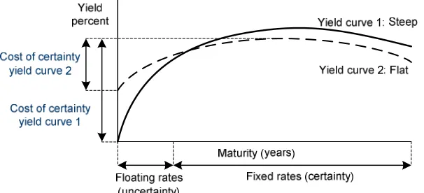
fixed-rate mortgage without penalty. The incentive is expected to depend, among others, on the yield curve

shape and on the increase in mortgage interest rate that clients are willing to suffer in order to obtain

the certainty that a fixed-rate mortgage offers.

1

These mortgages have interest rates (client rates) that fluctuate according to the Euribor rate but are offset with a fixed additional spread, which covers the bank’s costs and the profit margin.

2

[image:9.595.72.375.73.211.2]

October 2010 9

Figure 1: The cost of obtaining certainty by switching to a fixed-rate mortgage depends on the yield curve shape.

Because previous research projects were mainly focused on the refinance incentive (caused by

decreasing interest rates) for fixed-rate mortgages the conclusions and drivers cannot be copied on a

one-to-one basis, to floating-rate mortgages. Moreover, the absence of prepayment penalties in these

floating-rate mortgages affects the clients’ incentives to refinance.

This paper is intended to give insight into clients’ prepayment behaviour in a specific portfolio of

roll-over (floating-rate) mortgages to identify the variables that have driven the past prepayments (i.e.

prepayment drivers or explanatory variables).

“Why would someone prepay a floating-rate mortgage?”

Before prepayment analysis is initiated, preliminary research has been conducted to clarify the context

of the problem and the core problem. This preliminary research can be found in Appendix I and helps

to give insight to those readers not familiar with the risks of prepayments in general (a.o. fixed-rate

mortgages). Furthermore it explains explicitly which risks are posed by a prepayment for floating-rate

mortgages with fixed spreads.

In the next subsection “Problem analysis” the conclusions from the preliminary research are

summarized by answering the following two questions:

I. What are the main risks involved in a portfolio of floating-rate mortgages with a fixed spread over

Euribor?

II. How are these risks hedged and how could a prepayment function facilitate this, if forecasts of

October 2010 10

1.3. Problem analysis

The key issues in prepayment risk, that result from the preliminary research in Appendix I, are:

1. Funding spread volatility in combination with the long funding tenor (fixed spread is locked in)

which, unlike the Euribor interest rate, cannot be transferred onto the client after the

fixed-interest-rate period.

2. Reinvestment of prepayment proceeds occurs at a shorter tenor than the initial funding tenor.

3. Projections are not altered, because prepayment drivers are unknown.

Cash flows on funding Receipts from clients

Cash flows on funding Receipts from clients

FTP spreads drop. Client prepays

Cash flows on funding

Receipts from clients and re-investment

Re-investment of prepayment proceeds

Loss in income Margin New margin on re-investment FTP spread Euribor

1. Initial situation: contractual cash flows

2. Prepayment by client

3. Re-investment of prepayment proceeds

Prepayments: Re-investment risk in floating-rate mortgages

Initial cash flow profile with positive profit margin.

Client prepays and pays no future coupons. The coupon payments on funding still have to be made.

Due to a drop in FTP spreads the re-investment of the prepayment proceeds yields coupons that are too low.

It can be seen that when funding has high FTP spreads locked-in and FTP spreads drop, prepayment

by a client poses a risk. The proceeds from prepayment cannot be re-invested at sufficient interest

rates (sufficiently high spread over Euribor) to offset locked-in funding rates completely. A loss is

consequently incurred. It should be noted that a prepayment directly after an increase in FTP spreads

October 2010 11 1.3.1. Core problem identification

The final core problem identified is the issue that should be dealt with in order to tackle the observed

problem. The observed problem is the gains and losses arising from funding adjustments. The link

between the core problem and the observed problem is depicted in the causal chain below.3

1.3.2. Problem statement

Changing costs of liquidity, as defined by the FTP spread, can trigger economic losses when higher or

lower prepayments rates occur than were expected. As opposed to fixed-rate mortgages

re-investment risk applies to the entire remaining contract tenor, instead of only to the remaining time

until re-pricing at the moment the fixed-interest-rate period ends. To accurately project prepayment

rates CMRM first requires insight into the factors that drive these prepayments and the strength and

[image:11.595.71.335.174.294.2]

nature of their impact.

Figure 2: In the above model for the problem statement the nature, strength and direction of relationships between explanatory

variables and the independent variable are unknown.

3

October 2010 12 1.3.3. Problem owner and stakeholders

Problem owner

Transferring the liquidity- and interest rate risk to FM ALM is the task of CMRM. CMRM is the problem

owner when it comes to modelling these risks accurately.

Stakeholders

CMRM and business units: hedge ineffectiveness may lead to Profit & Loss volatility at the business

units and possibly to losses.

The entire bank: a wrong assessment of risk can lead to i) Economic Capital levels which are

insufficient to cover shocks, ii) pricing being too low leading to clients not being charged for the risk

they impose on the bank, iii) charging clients insufficiently for the prepayment option (and

corresponding potential gains) they receive.

1.3.4. Conclusions preliminary research

I. What are the main risks involved in a portfolio of floating-rate mortgages with a fixed spread over

Euribor without prepayment penalties?

Although the ever-changing Euribor component from the client rate in a floating-rate mortgage is

exactly charged onto clients every month by adjusting the client interest rate. The other components,

however, cannot be adjusted whenever they change, leading to the risk that some of these costs are

not compensated for in case of unexpected high or low prepayment rates.

For a portfolio, with relatively low liquidity (FTP) spreads locked into client rates, the main risk lies in

lower-than-expected prepayment rates requiring extra funding to be attracted at prevailing (high)

liquidity costs (higher than clients are paying), constituting an economic loss.

For a portfolio with high liquidity (FTP) spreads locked into client rates, the main risk lies in

higher-than-expected prepayment rates requiring funding to be unwound at prevailing (low) liquidity costs

(lower than clients are paying), constituting an economic loss. A constant (high or low) FTP spread

does not pose a risk.

II. How are these risks hedged and how could a prepayment function facilitate this, if forecasts of

explanatory variables were available?

If insight in prepayment drivers led to accurate prepayment projections and accurate

cash-flow-replicating portfolios, than no funding adjustments would be required and the exact liquidity costs paid

October 2010 13 1.3.5. Research questions

The preliminary research has led to the formulation of the following research questions:

1. Which explanatory variables can be identified as drivers for full and partial prepayments during the

period Dec. 2006 - Apr. 2010?

1A. Which explanatory variables are suggested by the literature?

1B. Which explanatory variables are found to be significant for the fixed-spread floating-rate

mortgages?

2. Which models and drivers explain full and partial prepayments between Dec. 2006 and Apr. 2010

most accurately?

2A. Which functional form is most suitable to model prepayments and identify drivers?

2B. Should partial prepayments be modelled separately? Are the two models for full- and

partial prepayments significantly different?

The suitability and fit of the model will be determined by appropriate measures for the type of model

chosen (see subsection 5.2.3)

The next section addresses the research design. Section 3:”Literature research” addresses research

question 1A by analyzing previous research on explanatory variables and functional forms of

prepayment models, which are, however, mainly focused on fixed-rate mortgages. Descriptive

analysis of dependent and independent variables is conducted in section 4 in order to formulate

hypothesized relationships between variables and prepayments. The explanatory research conducted

in section 5 will answer the research questions 1B, 2A and 2B. Section 6 contains the conclusions and

October 2010 14

2. Research design

This section elaborates on the scope of analysis in subsection 2.1, it covers the research questions in

subsection 2.2, and subsection 2.3 and 2.4 cover the research design and the data requirements

respectively.

2.1. Scope

2.1.1. Prepayment types and level of analysis

A portfolio of roll-over mortgages with a fixed spread over Euribor is analyzed. The portfolio contains

contracts with the same fixed spread but with different start dates and contract characteristics. The

contracts and prepayments will, therefore, be analyzed at an individual level in order to eventually

explain prepayment rates at an aggregated level, i.e. the portfolio. This prevents the loss of

information. Prepayment rate changes could in that case be explained by portfolio composition

changes as well4.

Due to data restrictions trigger prepayments cannot be distinguished as a subset of the full

prepayments. Full and partial prepayments are identified separately at a contract level and, together

(expressed as a percentage of the aggregated notional), they form the dependent variables which are

to be explained and for which drivers are to be found. The data filters applied to obtain the prepayment

data can be found in Appendix III.

4

October 2010 15 2.1.2. Empirical vs. optimal-call approach

The above box shows two approaches to prepayment modelling explained by Pliska (2006). We have

adopted the empirical approach in this research because the goal of this research is to determine

drivers for prepayments. Eventually ING intends to use this to attract mortgage funding with a suitable

duration that mirrors the expected cash flows, subject to the expected prepayments instead of the

optimal prepayments. The model should consequently fit observed prepayment behaviour which might

be non-optimal, because prepayments can occur for non-financial reasons as well.

2.1.3. Credit mortgages vs. other mortgages

Credit mortgages are analyzed separately.These mortgages are offered to clients so that they have

credit available when needed, which can be prepaid at all times. Prepayment behaviour for these

mortgages is, consequently, expected to have more idiosyncratic (client-specific) explanatory

variables.

If not analyzed separately these mortgages might add to the unexplained variance in the dependent

variable because the omitted explanatory variables are unsuitable. The reason they are important is

because their credit needs (notional increase) might at times offset prepayments (notional decrease)

by other clients. On the other hand prepayments could be boosted when clients with a credit mortgage

October 2010 16

2.3. Prepayment analysis

2.3.1. Longitudinal design

Longitudinal design means the prepayment behaviour of a group of clients (portfolio of mortgages) is

monitored over time to identify drivers (explanatory variables). In this case the analysis is done

[image:16.595.83.495.189.224.2]

retrospectively with logged data.

Figure 3: The research design does not include a control Group. Retrospective data analysis is applied.

In Figure 3 the “O” signifies a measurement on the outcome variable, which in this case depicts

whether a client has prepaid or not (binary). The “X” signifies an event (the prevailing values of the

explanatory variables). Keeping the research goal in mind explains why a method such as time series

analysis is not evaluated as an option; it does not result in drivers, other than time and a lagged

dependent variable. Because the portfolio involves a great amount of contracts, and data is several

years old a questionnaire or interviews are too cumbersome to execute with the resources available.

The methods of regression analysis is thus adopted to answer the research questions.

Potential future control group

In June 2009 new roll-over mortgages were introduced and sold with a variable spread over Euribor.

The two portfolios (fixed-spread and variable-spread roll-overs) have approximately a one-year time

overlap5. In the future, with more data this portfolio could serve as a control group. This is especially

relevant for determining the sole impact of changes in the liquidity spread.

5

October 2010 17

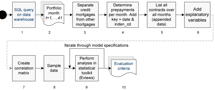
2.4. Prepayment data

The type of data determines, among others, the type of analysis and conclusions that are feasible.

This subsection addresses the origin of the data, the definition of a prepayment and the unit and level

of analysis.

2.4.1. Sources

The data are collected from the database HP. Prepayment data at a contract level of these mortgages

can be deduced from the databases as of December 2006.6

2.4.2. Data quality requirements

The data should be such that reliability and internal validity7 are sufficient and maximized. Several

factors are thus important with respect to the data:

- Time span covered: minimum of three years of prepayment data to cover variability in explanatory

variables.

- Contract age range: The portfolio consists of several contract ages (main part up to twelve years.)

- Yield curve changes (shifts, twists) observed during time span of prepayment data.

- Significant FTP spread changes observed during time span of prepayment data.

- Prepayment can be identified according to explicit definitions.

Variability in explanatory variables in the time span covered is crucial in regression analysis for

drawing reliable conclusions and maximizing internal validity of the research. The actual data that are

required and used and the prepayment definitions used are found in Appendix III. The amount of

contracts and amount of prepayment data is enormous and should not pose an issue for determining

whether explanatory variables are statistically significant or not.

2.4.3. Data quality assessment

The data obtained span a sufficiently long time period (41 months) and ages are well distributed over

the portfolio to meet the data quality requirements. See Appendix IV for information regarding the

distribution of contract start dates and reset periods.

Information regarding actual liquidity spreads, prepayment rates and portfolio sizes, is confidential and

has not been reported. Developments of these factors are shown, but in graphs without numbers on

the axes.

6 _{See Appendix III for the definitions of the different types of prepayments and the filter applied to obtain the data.} 7

October 2010 18

3. Prepayment drivers and functional forms

In this section literature research regarding prepayment analysis and corresponding explanatory

variables (prepayment drivers) is conducted in order to answer research sub question 1A. Potential

drivers following from this research will be analyzed in section 4 “Descriptive research” and tested for

their explanatory strength in section 5 “Explanatory research”. Literature about fixed-rate mortgages or

prepayments in countries other than the Netherlands will be assessed on relevance before it is

analyzed further.

Research question 1A:

Which explanatory variables are suggested by the literature?

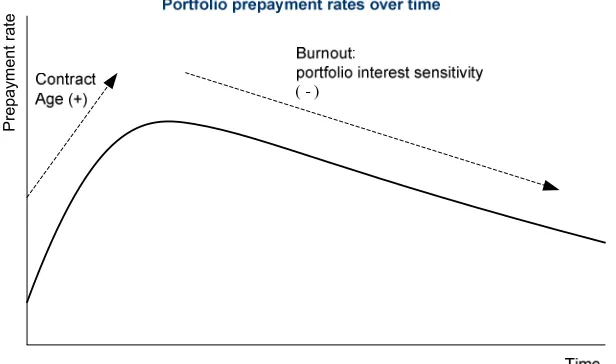
Definition: Seasoning vs. burnout

These concepts are addressed in the literature and, therefore, explained upfront. Seasoning refers to

the ageing of an individual client’s contract. Directly after taking on a new mortgage clients tend to

show low prepayment rates, but these increase gradually over time as the contract ages.

Burnout, on the other hand, refers to an ageing mortgage pool that exhibits decreasing rates of

prepayments, supposedly, because interest-rate-sensitive clients tend to prepay earlier and are

therefore less and less represented in the ageing pool. The older mortgage pool is therefore biased

towards interest-insensitive clients.

As is seen the contract age tends to dominate the prepayment rates initially, but over time the factor

burnout becomes more prevalent. Especially for a portfolio that has no new production inflow of

mortgages, as is the case for the fixed-spread floating-rate mortgages, the burnout effect is important.

P

re

p

a

y

m

e

n

t

ra

te

[image:18.595.73.381.546.728.2]

October 2010 19

3.1. Research into explanatory variables

3.1.1. Previous ING research:

The conventional explanatory variable that is used for fixed-rate mortgages is the interest spread (as a

proxy for the refinance incentive) between the client rate locked-in in the mortgage and the five-year

SWAP-FTP rate.8 ING introduces a three-month-lagged SWAP-FTP rate to compensate for the client’s

reaction time to interest rate changes. Previous research of Fanciulli (2009) has resulted in several

additional significant explanatory variables:

“The data present in at least two instances a very compelling case for (…):

1. Relative age of fixed interest rate period.

2. Initial notional”

The parameters of the prepayment function are not necessarily the same for different business units,

due to a potential difference in “financial sophistication” of clients, which is actually observed in

prepayment data of ING. The hypothesis is that financially sophisticated (e.g. educated) clients are

more aware of prepayment benefits when they occur than others.

Application to roll-over mortgages

The relative age might be a relevant explanatory variable in case of roll-overs.9 The interest spread for

roll-overs could be defined as the spread between a long-term fixed rate and the client rate (short-term

floating). A positive spread would constitute an incentive to switch from a roll-over mortgage to a

fixed-rate mortgage.

8 _{The SWAP-rate is the rate at which interest swaps are settled, but where the loan notional never flows to a counter party. The}

SWAP-FTP rate is based on the SWAP-rate but includes the costs of liquidity, because the notional is transferred as well.

9

October 2010 20 3.1.2. Mortgage prepayments in the Netherlands

Alink (2002) analyzes prepayments for fixed-rate mortgages (Appendix V). He suggests refinance

incentive, burnout, seasoning, and seasonality to be investigated. Refinance incentive is defined as

the difference between the client rate locked in and the prevailing market rate, dampened by potential

penalties. Seasonality refers to seasonal differences in prepayment rates.

The part of burnout that takes into account the heterogeneity of clients in a mortgage pool could be a

significant explanatory variable for this portfolio of roll-over mortgages.

initial t balance n

i n

i t

Pool Pool

Notional Notional

PF ,

1

i initial, 1

t i, g, outstandin

= =

∑

∑

=

= 0≤PF_t ≤1 t≥0

This method, however, has significant weaknesses because analysis occurs at a pool (aggregated)

level. It does not group individual clients, based on identified differences, fast prepayers and slow

prepayers (heterogeneity) to monitor the portfolio composition. On the contrary, using the pool factor

assumes that the fraction of fast prepayers decreases over time. If this is, however, not the case the

variable will simply turn out to be an insignificant driver after analysis. An alternative burnout proxy is

constructed and listed in Appendix VIII.

3.1.3. Prepayment risk in adjustable-rate mortgages subject to initial discounts

Ambrose & LaCour-Little (2001) state the following:

These comments concern yield curve characteristics, which are elaborated on in research

summarized in the next subsection. The authors go on to say that they incorporate the age of a

contract to account for seasoning and they include the quadratic term age-squared to “control for

nonlinearity in the shape of the hazard function”, which, however, risks introducing multi-collinearity

October 2010 21

3.2. Research into yield curve characteristics

One of the options to a client with a roll-over mortgage is to switch to a fixed-rate mortgage with a fixed

interest rate period of, for example, five or ten years. An interest rate corresponding to a single tenor is

in that case no longer sufficient to quantify refinance incentive. An entire range of tenors and

corresponding interest rates (a yield curve) may in that case impact clients’ prepayment behaviour.

Using the yield curve in explaining prepayments requires identifying explanatory variables10. This

subsection discusses the characterization of yield curves in order to use the characteristics as

explanatory variables instead of all the individual interest rates.

3.2.1. Curvature, level and steepness

In ‘Common factors affecting bond returns’ Litterman & Scheinkman (1991) identify common

explanatory variables that affect the returns on U.S. government bonds and related securities. It is

concluded that: “most of the variation in returns on all fixed-income securities can be explained in

terms of three factors, or attributes of the yield curve, which we will call level, steepness, and

curvature.”

Y

ie

ld

p

e

rc

e

n

t

10 _{Using individual interest rates corresponding to a range of tenors is undesirable since it would result in a large prepayment}

October 2010 22 Curvature

“The third factor, which we call curvature, increases the curvature of the yield curve in the range of

maturities below twenty years; the effect on yields tails off above twenty years.” (Litterman,

Scheinkman, 1991). Litterman, Scheinkman, and Weiss (1991) found that changes in curvature of the

yield curve have a relationship to the changes in rate volatility. Prices of fixed-income securities with

embedded options, such as callable bonds, are sensitive to this volatility.

A roll-over mortgage has such an embedded option as well, namely the option to prepay. Low

long-term interest rates in combination with a flat or inverted yield curve might induce clients to switch their

mortgage from floating-rate to fixed-rate in order to lock in these low rates and reduce uncertainty (due

to interest rate volatility) in their monthly instalments.

Christiansen & Lund (2005) suggest a specific butterfly spread (Appendix VI) as a measure of

curvature. An extra remark is made that w should be chosen such that the duration of the entire

butterfly spread is zero. The butterfly spread is given by: c_t = y_2t −

(

wy_1t+

(

1−w

)

y_3t

)

. The bond tenors y1, y2, and y3 have been chosen by the authors such that the final curvature measure (historically)

has a strong relationship (correlation) to interest rate volatility. The concluded tenors are three months,

three years and ten years respectively.

Level

“(…) the first factor represents essentially a parallel change in yields (…)” (Litterman, Scheinkman,

1991). As a measure of level, Christiansen & Lund (2005) recommend using the three-month yield,

stating: “The 3 month yield is applied as a proxy for the instantaneous short term interest rate, and in

our analysis it corresponds to the level of the term structure;l_t =y_1t”. The variable y1t corresponds to their variable used in the measure for the curvature.

Steepness (slope)

“(…) a shock from the steepness factor (as defined here) lowers the yields of zeroes up to five years,

and raises the yields for zeroes of longer maturities.” (Litterman, Scheinkman, 1991). As stated,

changes in steepness (slope) can be observed by a changing spread and a decreasing slope may

pose an incentive for clients to switch from a floating- to a fixed-rate mortgage.

Moreover, Litterman, Scheinkman, and Weiss (1991) suggest that a high slope is an indicator of

expectations for interest rates to rise. To determine a measure of the slope Christiansen & Lund

(2005) state the following: “In the empirical analysis, the slope of the yield curve is defined by

t t

t y y

s = ₃ − ₁ (…)”11. The variables y1t and y3t correspond to the ones used in measuring the curvature.

11 _{The reason the authors state is: “(…) in terms of keeping the correlation between the slope and the butterfly spread at a}

October 2010 23

3.3. Research into prepayment models: functional forms

This subsection addresses three papers that address proportional hazard models to explain

prepayment rates. These models have the form λ

( )

t;z =λ₀

( )

tezβintroduced by Cox (1972)12. The hazard rate, variableλ

( )

t;z , depicts the expected fraction of clients that will prepay in a given time period. All three articles apply baseline hazards,λ₀

( )

t , which are boosted or dampened by proportionality factors, ezβ, which depend on the values of explanatory variables z, and the

coefficients β. The entire model, therefore, accounts for the dependence of the hazard rate,λ

( )

t;z , on explanatory variables.

Parametric assumptions about the distribution of the survival time and consequently the hazard rate

have thus been made before estimation of the parameters starts. Besides the proportional hazard

models, this subsection covers Logit, Probit and Extreme Value models as well.

( ) ( ) ( )

t = f t /S t λ

3.3.1. Prepayment Behaviour of Dutch Mortgagors

Charlier and Van Bussel (2001) performed a study on fixed-rate mortgages in the Netherlands. They

apply an S-shaped seasoning curve, and use the following proportional hazard model:

(

)

(

)

it t x z it age t e z e x e age h ' ~ . 2 1 0 , ~ ; 1 1 , ; 2 1 υ υ υ υ π υ υ − − − − = = + =

(

_;υ _,υ

) (

_.π _;υ~

)

2

1

0 t it

it h age x

h =

(

υ

)

π _;~ it x it

x υ~

υ~ it h 12 t

October 2010 24

The functional form of

π

(

x

_it

;

υ

~

)

reflects the extreme-value distribution which can be used to estimate

binary models. The functionial form of

h

₀

(

age

_t

;

υ

₁

,

υ

₂

)

reflects a logistic function (Logit model). The

authors analyzed four explanatory variables: refinance incentive, burnout, seasoning and seasonality.

For savings and interest-only mortgages it is among others concluded that “the likelihood that a (…)

mortgage will be prepaid increases with the age of the mortgage. Models excluding burnout also lead

to a positive relationship between prepayments and the refinance incentive. However, when burnout is

included the direct effect of the refinance incentive disappears and is taken over by burnout.”

3.3.2. Mortgage Prepayment Behavior in a Market with ARMs only

He & Liu (1998) have performed a study on ARMs (Adjustable-rate-mortgages) in Hong Kong.

(

)

(

)

v e t v

t θ π γ ρ β

π ; ; = ₀ , , .

(

)

( )

( )

p p t t p p t γ γ γ γ π + = − 1 ; ; 1 0 0 = v * t

(

)

γ p p t / 1 1 *= −

( )

(

) ( )

(

( )

)

( )

( )

(

( )

)

( )

(

( )

)

∑

∑

∑

∑

∑

= = = = = +         −         +         − + + − − + + = J j p i s h i h h I i s h p i s h i h h i h h p i i t t v t t v t v t t p L 1 1

1 1 1

1 ln exp 1 ln exp 1 ln ln 1 ln ln ln γ β γ β β γ γ ρ γ θ

This baseline hazard function shows the prepayment rates in the absence of explanatory variables’

influences other than age (“homogenous conditions”). The above description of the baseline hazard

seems to indicate that the seasoning effect that is accounted for, implicitly takes burnout into account

October 2010 25

3.3.3. Mortgage Prepayment and Default Decision: a Poisson Regression Approach

Schwartz & Torous (1993) apply the proportional hazard function as well, but suggest Poisson

distributed events. This justifies Poisson regression. Their study involves geographically dispersed

fixed-rate mortgages in the United States.

(

)

, 0,1,2,... !

)

( = =

=

= − x

x e x f x X P

x π π

( )

θ π= v,

( )

[

_vt

]

(

)

_eβπv( )t π π

π β π τ α

α τ

π , , , = ₀ ,

The difference with the log-logistic baseline hazard of He & Liu (1998) is thus the way time

dependency is modelled. Schwartz & Torous (1993) divide mortgage contracts over age-buckets and

estimate constant baseline hazards for each bucket, whereas He and Liu use a log-logistic function to

account for the entire range of ages in the portfolio.

3.3.4. Probit, Logit and Gumbel regression

Hosmer & Lemeshow (2000) and Cramer (2003) discuss the application of the Logit and Probit model

and the interpretation of the model results (see User’s guide Eviews 6 as well). This subsection

summarizes some of their conclusions and discusses Gumbel regression as well.

“Whereas the hazard function in continuous time is defined as the instantaneous rate of failure

conditional on survival to a given point in time, the discrete-time hazard is the probability that an event

occurs (…) in the interval from t to t +1 , given that an event has not already occurred prior to t”

[Calhoun, Deng, 2000]. A prepayment either occurs or does not in a specified month.

Probit, Logit and Gumbel models are meant for these kinds of binary dependent variables, because

they address the issue of the bounded outcome values, whereas inputs are unbounded. The predicted

values are bounded between zero and one by transforming a linear equation

k kX X

X β β

β

β0+ 1 1+ 2 2+...+ with range

(

−∞,∞

)

to a range

[ ]

0,1. This transformation is done through the use of a cumulative distribution function.

These binary models do not require the assumption of normality with respect to the residuals of the

regression analysis. Statistical tests on coefficients are thus valid even if errors are not normally

October 2010 26

(

) (

)

(

1| 0, 0

)

( )

0 0.5

... , ,..., , | 1 0 , , , , , 2 2 , , 1 1 0 , , , , 2 , , 1 , = Φ = = = = + + + + Φ = = β β β β β x β t i t i k k t i t i t i k t i t i t i y P x x x x x x y P

(

)

( )

(

)

0.5

1 1 0 | 1 ... 1 1 , ,..., , | 1 0 , , , , , , , 2 2 , , 1 1 0 , , , , , , 2 , , 1 , = + = = = + + + + + = + = = − − e y P x x x v e x x x y P t i t i t i t i k k t i t i t i t i v t i k t i t i t i v β ε β β β β

(

)

(

( )

)

(

)

(

1| 0, 0

)

exp

(

exp

( )

0

)

0.37 ... exp exp , ,..., , | 1 1 0 , , , , , 2 2 , , 1 1 0 , , , , , , 2 , , 1 , ≈ = − = = = = + + + + = − − = = − e y P x x x v v x x x y P t i t i k k t i t i t i t i t i k t i t i t i β β β β β x β Φ t i

v_, pi,t /

(

1−pi,t

)

( )

(

odds

)

p p v p Logit t i t i t i t i ln 1 ln , , , , _=       − = =

(

1−pi,t

)

The asymmetry of the distribution and the fact that it is intended to model extreme events make the

Extreme-Value model less suitable than Probit and Logit models. For logistic regression the odds ratio

helps interpreting final model results and its drivers. It is a measure of association of odds instead of

probabilities. The odds ratio is explained in the following example:

( )

(

)

(

)

( )

(

)

(

)

2.01 1 / 1 / 1 1 1 / 1 1 1 / 1 1 1 70 . 0 0 0 1 , ≈ = − − = = =       +         +       +         + =        − = = − = = + = = = = = − + + + + + + + + = = = = e p p p p ratio Odds e e e e e e e e e ratio Odds p p b x Odds p p a x Odds x c p Logit x x x x b a b c a c b c b c b c a c a c a c b x b x a x a x t i β β β β β β β β β β } 96 . 1 ˆ { : .

October 2010 27

3.4. Distinction among types of prepayments

Research question 2B

Should partial prepayments be modelled separately? Are the two models for full- and partial

prepayments significantly different?

No literature was found that aims to model partial prepayments separately from full prepayments. This

might be because of practical considerations resulting from the typical relatively small part of the

portfolio that partial prepayments make up, as measured in currency.

The distinction is relevant in case these prepayments have different drivers. This may be likely if one

considers a partial prepayment as an investment with a risk-free rate of return equal to the mortgage

client rate. If the mortgage client rate exceeds alternative risk-free investments in the market then

clients in this portfolio have the incentive to prepay partially13. The benefit is reduced by the tax rate,

because of deductibility of mortgage interest payments. Lowering of tax deductibility in combination

with low short-term interest rates, might consequently induce partial prepayments.

Extracting the partial prepayment data from the full prepayment data prevents these data from

clouding the regression analysis on full prepayments. Eventually this may lower the unexplained

regression variance, which is our goal.

Although there might be a practical consideration not to estimate two separate models (partial

prepayments rates are relatively low), the academic question “Are the two models for full- and partial

prepayments significantly different?” remains, and will be further addressed in section 4 and 5.

13

October 2010 28

3.5. Conclusion

Partial prepayments in particular may have other drivers than full- and trigger prepayments. For this

reason partial prepayments are analyzed separately in the descriptive- as well as the explanatory

research. Trigger prepayments are not distinguished from other full prepayments, because of

restrictions in data structure.

Two separate models are, therefore, constructed in order to reduce the unexplained variance in the

regression results. A hypothesis test will be performed to test the statistical significance of the

difference between the model for partial- and the model for full prepayments which will answer

research question 2B.

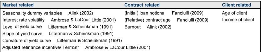
Research question 1A: Which explanatory variables are suggested by the literature?

To characterize yield curves the characteristics level, slope, and curvature, as defined by Christiansen

& Lund (2005), are used in subsequent sections. Other suggested prepayment drivers are relative

contract age (seasoning), seasonality, level, slope, curvature, burnout and interest rate volatility.

Moreover, it is hypothesized that clients with high incomes and a high initial loan notional are more

likely to prepay than others. Besides the definition of burnout according to Alink (2002) a second

definition will be used to investigate the burnout’s explanatory strength (Appendix VIII).

Burnout’s importance in this particular portfolio comes from the fact that no inflow of new mortgages

will occur, meaning that the portfolio size will slowly decrease and any burnout effect in prepayment

rates would not be compensated for by new mortgages entering the pool.

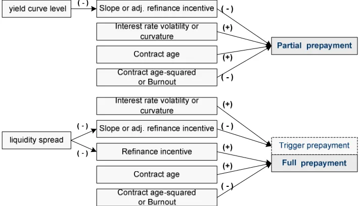
Unique for floating-rate mortgages are Interest rate volatility and slope. Both variables are expected to

be related to switches from floating-rate to fixed-rate mortgages, assuming a fixed-rate mortgage is

[image:28.595.72.527.534.624.2]

perceived as a haven of certainty as opposed to a highly volatile floating-rate mortgage.

Figure 5: The variables that will be investigated further in section 4 and 5.

Proportional hazard models and binary response models such as Logit, Probit and Gumbel were found

to model prepayments. To make a final model choice, the empirical distribution of prepayments is first

observed in section 4. Section 5 contains a further analysis and overview of the beneficial aspects of

October 2010 29

4. Descriptive research

In this section the historical values and developments of potentially relevant explanatory variables are

investigated and the dependent variables. This serves several goals:

1. The empirical distributions of the dependent variables influence the choice (suitability) of the

prepayment’s functional form.

2. Historical developments are analyzed to check whether sufficient variability in explanatory

variables has been present in the time period covered.

3. A pair-wise correlation matrix is constructed to identify potential sources of multi-collinearity.

4. Preliminary insight is obtained into potential relationships between explanatory variables and the

dependent variables.

Research question 1B:

Which explanatory variables are found to be significant for the fixed-spread floating-rate mortgages?

The insight this section gives will help formulate hypothesized relationships to be tested in section 5,

which will consequently answer research sub question 1B.

Subsection 4.1 addresses the historical prepayments and their empirical distribution, which form the

basis for the choice of a suitable prepayment function in section 5 “Explanatory research”. Subsections

4.2 and 4.3 cover the historical developments of explanatory variables and their pair-wise correlations.

Subsection 4.4 summarizes the conclusions drawn from the literature research and the descriptive

research by formulating hypotheses graphically.

4.1. Historical prepayments

4.1.1. Empirical distributions

The prepayment rates will be analyzed as a fraction of contracts in the portfolio, which coincides with

the research goal to model and explain client behaviour. To investigate the portfolio impact, each

client’s probability of prepayment can be calculated with the corresponding outstanding notional.

Full prepayments

The overall portfolio prepayment rate for a certain month follows from individual contracts either

prepaying fully, partially, or not at all. If the partial prepayments are left out and analyzed separately,

October 2010 30 t i p_, t i p_, i,t x t t n X /

[

Xt nt

]

E /

[

]

[

*

]

. 1 , , g outstandin ,

∑

= = n i t i t i

prepaid p L

L E

t i L_{outstanding,,}

t i,t bernoullirv fori n x ~ .., =1,2,...,

, 1 , 0,1,..., n t i t t i X

x for t T

n

=

= =

∑

Partial prepayments

Partial prepayments do not lead a client to drop out of the portfolio, so n is unaffected, however, the

outstanding notional does decrease. Again the dependent variable is binary, since a client either

prepays (partially) or does not. Individual partial prepayments may again be dependent on one

another through common explanatory variables (drivers) although the impact of idiosyncratic factors

(surplus cash that is invested by prepaying partially) is expected to be greater. Whether or not a client

prepays is driven by drivers, whereas the amount that is prepaid is assumed to be more client-specific.

For this reason the fraction of clients prepaying is, just as for full prepayments, used as dependent

variable.

[

]

∑

[

[ ]

]

= = n i t i t i

Partial p E FL

L E 1 , , g outstandin , *

[ ]

F

E L_{outstanding,i,t} E

[ ]

F

[ ]

k M F E t n i t i 41 41 1 1 ,

∑∑

= = =

[ ]

F E

t i M _,

4.1.2. Historical prepayments

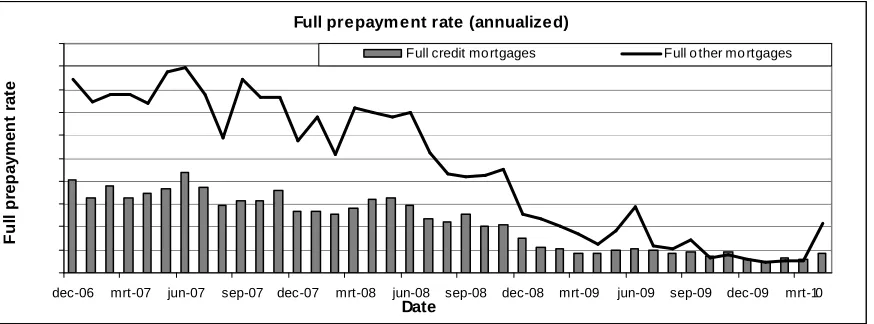
In Appendix VII the full and partial prepayment rates (as a fraction of the portfolio) for credit mortgages

and other mortgages are displayed in graphs. The actual prepayment rates are not depicted, but the

developments over time are visible. This subsection will summarize the preliminary findings obtained

October 2010 31 Full prepayments

While credit mortgages are expected to have different prepayment drivers the graphs displaying the

prepayment rates move seem to show the same movements. This suggests that they are strongly

impacted by a common driver, i.e. a common explanatory variable.

Full prepaym ent rate (annualized)

0% 5% 10% 15% 20% 25% 30% 35% 40% 45% 50%

dec-06 mrt-07 jun-07 sep-07 dec-07 mrt-08 jun-08 sep-08 dec-08 mrt-09 jun-09 sep-09 dec-09 mrt-10

Date

F

u

ll

p

re

p

a

y

m

e

n

t

ra

te

Full credit mo rtgages Full o ther mo rtgages

Figure 6: The full prepayment rates of source system HP are displayed. A distinction is made between credit mortgages and

other mortgages, because of their potentially different prepayment drivers.

Partial prepayments

A negative partial prepayment for credit mortgages means extra credit was drawn by the client from

the credit facility. The correlation (partial prepayments) for credit mortgages and other mortgages is

remarkably high with a correlation coefficient equal to 0.64.

Low partial prepayments intuitively are correlated to low interest rates, which is also a beneficial time

for clients with a credit mortgage to draw extra on their credit facility. Because of this positive

correlation hardly any diversification is obtained which is unfortunate for the overall portfolio variance.

Because the partial prepayments have a significant correlation with the full prepayments as well, with

a correlation coefficient of 0.57, the variability of the aggregated prepayments is hardly reduced.

Although the variance may not benefit significantly from diversification effects, the impact of

prepayments on the hedge portfolio is reduced by the negative partial prepayments of the credit

mortgages because they compensate for part of the partial and full prepayments of the other

mortgages, which are by definition positive. In short, when part of the prepayments is compensated for

[image:31.595.77.514.160.322.2]

October 2010 32

4.2. Historical values of explanatory variables

This subsection will discuss the historical developments of contract- and market-related variables, to

get a first indication of potential relationships that may exist with the prepayment rates in the same

period. Multi-collinearity will be addressed by analyzing pair-wise correlations.

4.2.1. Operationalization

For fixed-rate mortgages the main driver for prepayments is said to be refinance incentive (for

household relocation, which prevents a fine to be paid), which arises from decreasing market rates.

The equivalent for roll-overs is the refinance incentive that arises due to changes in the client spread

that is paid over Euribor.

Besides this, the incentive to switch from floating-rate to fixed-rate mortgage could arise from the

difference between a long-term fixed rate and the client rate (short-term floating). Clients may even

prefer a fixed rate (certainty) over a floating rate (uncertainty) whenever the ten-year-fixed rate is

slightly above the short-term floating rate. The resulting variable that measures the incentive to switch

to a fixed-rate mortgage is referred to as the adjusted refinance incentive. See Appendix VIII for the

operationalized explanatory variables.

Lagged explanatory variables

To account for the client's reaction time to interest rate changes a lag in the explanatory variables is

introduced. A big interest rate change is quickly noticed by a client with a floating-rate mortgage,

because of the consequent change in monthly instalments. Lags up to 5 months are investigated.

4.2.2. Contract-related variables

In Appendix IV it can be seen that the portfolio contains mortgages of all ages between 0 and 10 years

(1.7% is older). Appendix IX gives some insight into the developments of the average initial contract

notional over time.

4.2.3. Market-related variables

This subsection will give an overview of historical developments in market-related variables, namely

yield curve shape14 and Euribor short-term rates (height and volatility).

Liquidity spread (FTP): 2006 - 2010

The variability in the liquidity spread is the trigger that led to this research. A quick scan of the FTP

spread over time has indicated that liquidity costs have increased sufficiently during the credit crisis,

for them to be used as explanatory variable.

14 _{In subsection 3.2.: “Research into yield curve characteristics”, the method of measurement of level, slope, and curvature has}

October 2010 33 Yield curve shape: Jan. 2006 – Jun. 2010

Client rates are based on the SWAP-FTP curve but contain risk spreads and the profit margin as

well15. Even though clients observe client rates offered in the market, the use of the SWAP-FTP curve

(and its characteristics) as explanatory variable is accurate as long as the spread between both is

relatively constant.

During and after the credit crisis, however, the discrepancy of the five-year SWAP-FTP rate and the

five-year mortgage client rate has grown. Projecting prepayment rates based on the SWAP-FTP

projections might in that case lead to overestimating prepayment rates, whereas a future decrease in

the discrepancy will most likely result in underestimates of the prepayment rates.

Over the period 2000-2010 several yield curves shapes are observed which are summarized by using

the characteristics level, slope, and curvature in Figure 7. As can be seen the actual level of interest

rates has varied significantly as well as the shape. The variability is even greater when quarterly or

monthly data is analyzed. It should be noted that level and slope have a high inverse relationship,

which follows from their definition16.

Historical yield curve characteristics

-60% -30% 0% 30% 60% 90% 120%

Jan. 2000 Jan. 2001 Jan. 2002 Jan. 2003 Jan. 2004 Jan. 2005 Jan. 2006 Jan. 2007 Jan. 2008 Jan. 2009 Jan. 2010

Yield curve date

M

e

a

s

u

re

-4% -2% 0% 2% 4% 6% 8%

Curvature (left axis) Level Slo pe

Figure 7: Observed yield curve (SWAP-FTP) characteristics between 2000 and 2010. Characteristics are ‘level’, ‘slope’, and

‘curvature’. Measurement moments are the first available curve of January and June of each year.

15 _{The reason SWAP-FTP is practical is its easy availability and because projections of it can be modelled by Hull-White interest}

rate models, which consequently serve as inputs to project future prepayment rates. Modelling market client rates would require projecting future risk spreads and profit margins as well.

16 _{They both depend on the three-month rate. Although the slope depends on the ten-year rate as well, this rate is far less}

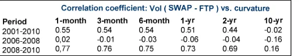
[image:33.595.79.512.384.536.2]

October 2010 34 Interest rate volatility vs. Curvature

The relationship between curvature of the yield curve and the interest rate volatilities of different reset

periods is shown in Appendix X. From the correlation coefficients in Figure 8 it can be seen that the

supposed relationship by Litterman, Scheinkman, and Weiss (1991) between the curvature and the

interest rate (SWAP-FTP) volatility has been quite strong over the period Jan. 2008 - Jun. 2010 and

weak over the other periods. The highest correlation is found with the short rates, the three-month,

six-month and one-year SWAP-FTP interest rates.

Figure 8: The table shows the correlation coefficient between the volatility of different SWAP-FTP rates with the curvature

measure for different time periods.

4.3. Pair wise correlations

Multi-collinearity clouds the individual explanatory variables’ impact on the dependent variable and is

caused by highly correlated explanatory variables. For this reason pair wise correlations have been

investigated for the data samples. Appendix XI shows the correlation matrix.

4.4. Conclusion

The full and partial prepayment rates have varied substantially over the period analyzed. As expected

prepayment rates have shown a declining trend due to the decreasing short term rates and the

increasing yield curve slope. The value of full prepayments is far higher than that of partial

prepayments, making them the most important ones to explain by drivers.

The yield curve shape, as defined by level, slope, and curvature, as well as the other explanatory

variables have shown sufficient variability over the time period 2006-2010, in order for them to be used

in regression analysis. Due to high correlations among explanatory variables, they cannot all be used

[image:34.595.74.378.210.267.2]