Mixing, Chemical Reactions, and Combustion in Supersonic Flows

Mixing, Chemical Reactions, and Combustion in Supersonic

Flows

Thesis by

Niccolo Cymbalist

In Partial Fulfillment of the Requirements for the Degree of

Doctor of Philosophy

California Institute of Technology Pasadena, California

2016

Acknowledgements

First and foremost, I would like to thank my advisor, Paul Dimotakis. In addition to providing me with ample resources, technical mentorship, and encouragement when the ‘going got tough’, he gave me a comprehensive education that extends well beyond science and engineering.

I would also like to thank Daniel Lang, whose optics and electronics expertise was critical to the success of the experimental portion of this work.

I very much enjoyed collaborating with Graham Candler on the development of LES-EVM. Seeing the project come to fruition was immensely fulfilling. I also enjoyed working with Elizabeth Luthman on the schlieren image-correlation velocimetry and chemically reacting experiments. Her good humor and attentive eye during the long days spent in the lab are particularly appreciated.

I’d like to thank the machine shop for their fabrication help, as well as Bahram Valiferdowsi and Prakhar Mehrotra, who assisted in the early stages of the experimental work.

Abstract

Experiments were conducted at the GALCIT supersonic shear-layer facility (S3L) to investigate aspects of reacting transverse jets in supersonic crossflow using chemiluminescence and schlieren image-correlation velocimetry. In particular, experiments were designed to examine mixing-delay length dependencies on jet-fluid molar mass, jet diameter, and jet inclination.

The experimental results show that mixing-delay length depends on jet Reynolds number, when appropriately normalized, up to a jet Reynolds number of 5×105_{. Jet inclination increases the}

mixing-delay length, but causes less disturbance to the crossflow when compared to normal jet injection. This can be explained, in part, in terms of a control-volume analysis that relates jet inclination to flow conditions downstream of injection.

List of Figures

1.1 Three-dimensional schematic of a transverse jet in supersonic crossflow (TJISCF), from Gruber et al. (1995) . . . 20

2.1 Gas-delivery system diagram (Bond 1991, Fig. A.1) . . . 25

2.2 Test-section dimensions, in inches . . . 26

2.3 RN1 (dj = 0.20 in., left), RN2 (dj = 0.25 in., center), and RI1 (dj = 0.25 in., right)

injector-orifice geometry . . . 27

2.4 Optical system combining schlieren/shadowgraph (right-propagating light), and chemi-luminescence (left-propagating light, diagram not to scale) . . . 29

2.5 Image A (top), and image B (bottom), ∆tIF= 6µs (Run ss1694) . . . 30

2.6 Streamwise velocity component of convected refractive-index interfaces of a helium jet in supersonic nitrogen crossflow (Run ss1694) overlaying a shadowgraphy image of the same flow . . . 31

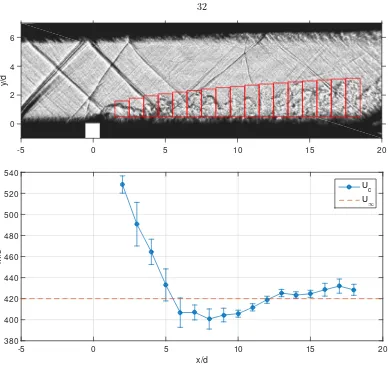
2.7 Binning structure (top) used to produce average convective-velocity estimates (bottom) of Run ss1694. Error bars mark the standard deviation (±σ) of the measured convective velocity within the bin. The freestream velocity is estimated as U∞= 420 m/s. . . 32

2.9 Velocity magnitude slice (left), jet-fluid concentration slice (center), and conditional velocity slice (right), derived from the LES results by E. Luthman. The YHe = 0.1

contour is outlined in red. . . 34

2.10 Binned SICV measurements using simulated-shadowgraph image pairs, and velocity magnitude of fluid with a jet-fluid mass-fraction of 0.1< YHe<0.9. Uncertainty bars

in the SICV estimates mark the±σestimated convective velocity within each bin. . . 34

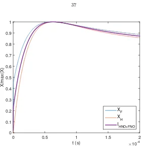
2.11 Normalized atomic fluorine and hydrogen mole fractions, and estimated average HNO*+NOF* chemiluminescence in a homogeneous reactor, assuming equal contributions from each species . . . 37

2.12 Typical reacting TJICF chemiluminescence image showing the mixing-delay length and jet body (Run ss1708) . . . 38

2.13 Chemical timescale for M1 and M2 mixtures, defined as the time at 0.6 of maximum chemiluminescence. See text for details. . . 39

2.14 Chemiluminescence, Ilum, and temperature rise, ∆T, normalized by the adiabatic,

equilibrium temperature rise, ∆Tf, for mixture M1 in Table 2.2, at T0 = 200 K, and

p0= 1 bar. . . 40

2.15 Overlayed time-averaged chemiluminescence and schlieren image (Run ss1708) . . . . 41

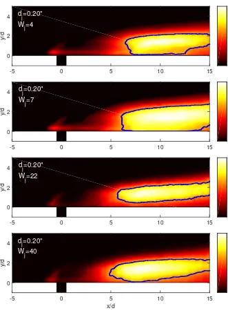
3.1 From top to bottom, chemiluminescence images of Runs ss1708 (helium jet), ss1714, ss1718, and ss1722 (argon jet). The mixing-delay length decreases with increasing jet-fluid diluent molar mass,Wj. The colorbar scale ranges from 0 to 1 and corresponds to

the chemiluminescence intensity normalized by its maximum value. The blue contour is the 0.6 locus of the maximum chemiluminescence signal. . . 45

3.2 Jet-fluid molar-mass effects on mixing-delay length. Uncertainty bars represent the individual measurement uncertainties discussed in Section 2.2.2. . . 46

3.4 Shear-layer velocity ratio (top left), convective velocity with measured TJISCF near-jet convective velocity (top right), growth rate (bottom left), start of mixing transition (Reδ >104, Konrad 1977, Dimotakis 1991, 2000) in jet diameters, fordj=0.2 in.

(bot-tom right) . . . 49

3.5 From top to bottom, chemiluminescence images from$= 4.11 (He+N2 jet fluid) Runs

ss1714,dj = 0.20 in. (top) and ss1719, dj= 0.25 in. (center top), from$= 0.66 (Ar

jet fluid) Runs ss1722,dj= 0.20 in. (center bottom) and ss1720,dj= 0.25 in. (bottom). 53

3.6 Mixing-delay length normalized by the physical orifice diameter plotted against jet Reynolds number. The uncertainty bars reflect the estimated measurement uncertainty discussed in Section 2.2.2. . . 54

3.7 Mixing-delay length normalized by jet-source diameter plotted against jet Reynolds number. The uncertainty bars reflect the estimated measurement uncertainty discussed in Section 2.2.2. . . 55

3.8 Mixing-delay length criteria of 0.5 (green), 0.6 (blue), and 0.7 (magenta) of maximum chemiluminescence signal . . . 56

3.9 Mixing-delay length normalized by jet-source diameter plotted against jet Reynolds number, for mixing-delay length criteria of 0.5, 0.6, and 0.7 of the maximum chemilu-minescence signal. Uncertainty bars omitted for clarity. . . 57

3.10 Chemiluminescence images from$= 4.11 Runs ss1714,tchem= 21µs (top) and ss1712,

tchem= 10µs (bottom). . . 58

3.11 Chemiluminescence images from Runs ss1719, normal jet (top) and ss1724, 30◦_inclined jet (bottom). . . 61

3.13 Average (binned) convective velocity from Runs ss1719 (normal jet), and ss1724 (in-clined jet). . . 63

3.14 Inclined jet-in-crossflow system . . . 64

3.15 Velocity, Mach number, total-pressure, and stream thrust function,Sa, change plotted against injection angle,θj . . . 66

4.1 Non-premixed hydrocarbon flame (left, Dimotakis 1997, reproduced with permission), and OH-PLIF in a burning ethylene jet in supersonic, heated O2 crossflow (right,

Ben-Yakar 2000, reproduced with permission) . . . 72

4.2 Premixed ethylene-air flame structure at combustor inlet conditions anticipated in a M∞= 6 scramjet . . . 74

4.3 Convected material element . . . 78

4.4 Product mass-fraction source term for various values ofχ, for a WSR entraining burnt fluid (top), and unburnt fluid (bottom) . . . 82

4.5 Radical-pool concentration-evolution predictions using detailed chemical kinetics . . . 87

4.6 Ethylene ignition radical-pool growth (UCSD mechanism) . . . 89

4.7 Decrease in maximum residual with iteration number k (solid black). The k-value cutoff is selected when the residual decay approaches a smooth curve (dashed red). . . 91

4.8 Reciprocal ignition-delay surface . . . 93

4.9 Residuals as a function of temperature (left) and pressure (right) . . . 93

4.10 Overall reaction rate plotted against the combustion-evolution variableτc, conditional

onZ and h, forτc,en∈[0,1] . . . 99

4.11 Fuel mass-fraction plotted against the combustion-evolution variable, conditional onZ andh, forτc,en∈[0,1] . . . 100

4.13 Definition of the overall reaction-evolution variable, τ, during the various stages of combustion. . . 104

5.1 LES-EVM interaction diagram . . . 109

5.2 Instantaneous OH mass fraction at the centerplane from an LES incorporating a flamelet model with compressibility corrections (Saghafian et al. 2015, Fig. 8, re-produced with permission), of the Gamba and Mungal (2015a) experiment (cf. Fig. 5.5) . . . 111

5.3 Hydrogen-air manifold discretization for the evolution-variable coordinateτ (top left), mixture fractionZ (top right), internal energye(bottom left), and densityρ(bottom right), in terms of the coordinate value plotted against the corresponding index. . . . 113

5.4 Left: H2O mass-fraction slices as a function of [Z, ρ, τ], with e= 0 J/kg. Right: H2O

mass-fraction slices as a function of [Z, e, τ], withρ= 0.5 kg/m3_{. . . . 114}

5.5 OH-PLIF image of the crossplane in a reacting hydrogen-air TJISCF, from Gamba (2015a), Fig. 9, reproduced with permission. . . 115

5.6 Centerplane OH concentration from an EVM-LES simulation of the G15a experiment. Figure based on LES data courtesy of G. Candler. . . 115

5.7 Experimental OH-PLIF image (top, Gamba 2015a, Fig. 18, reproduced with permis-sion) and simulated OH mass fraction (bottom, figure based on LES data courtesy of G. Candler.) on a plane parallel to the lower guidewall, aty/dj= 0.25. . . 116

5.8 Centerplane H2O mass fraction (top), and temperature (bottom) from the LES-EVM

simulation of the G15a experiment. Figure based on LES data courtesy of G. Candler. 118

5.9 OH contours for simulations with grid resolution of 14 million elements, with fourth-order spatial accuracy (top), and 70 million elements, with second-fourth-order spatial accu-racy (bottom). Figure based on LES data courtesy of G. Candler. . . 119

A.2 Average cross-correlation signalC¯ at a location in the jet wake region produced with 32 image pairs. xand y axes have units of pixels, while the z axis is the normalized cross-correlation coefficient, R, that ranges from -1 to 1 . . . 137

A.3 Four randomly selected sample individual cross-correlation signalsCn. xand y axes

have units of pixels, while thez axis is the normalized cross-correlation coefficient, R, that ranges from -1 to 1 . . . 138

B.1 Chemiluminescence system calibration curve illustrating a quasi-linear response. The x-axis is the normalized applied intensity, and the y-axis is the normalized measured intensity. . . 143

C.1 Comparison of various potential ignition criteria . . . 145

C.2 Logarithmic variance between recent chemical-kinetics mechanisms and experimental ignition-delay data plotted as a function of initial mixture temperature. The thick black line represents the variance between the proposed EVM method and experimental data. 147

C.3 Logarithmic variance between heritage chemical-kinetics mechanisms and experimental ignition-delay data plotted as a function of initial mixture temperature. The thick black line represents the variance between the proposed EVM method and experimental data. 148

List of Tables

2.1 Injector-block specifications . . . 27

2.2 Reacting-gas composition . . . 39

3.1 Jet-fluid molar-mass effects . . . 44

3.2 Jet-diameter effects . . . 52

3.3 Chemical-timescale effects . . . 59

3.4 Jet-inclination effects . . . 60

4.1 Turbulence-chemistry scaling in an ethylene-fueledM∞= 6 scramjet . . . 76

4.2 Detailed chemical-kinetic mechanisms . . . 85

4.3 Experimental (shock-tube) ethylene ignition-delay data sets . . . 86

4.4 Fit coefficients . . . 92

4.5 Mixture fraction,Z, example . . . 96

5.1 Gamba (2015a) experimental conditions . . . 112

Contents

Acknowledgements v

Abstract vi

1 Background and introduction 18

1.1 Reacting jet in supersonic crossflow . . . 20

1.2 Thesis objectives . . . 23

2 Experimental setup and diagnostics 24 2.1 Facility overview . . . 24

2.2 Diagnostics and data processing . . . 27

2.2.1 Schlieren image-correlation velocimetry (SICV) system . . . 28

2.2.1.1 Comparison with artificial shadowgraph SICV . . . 32

2.2.2 Nitrosyl fluoride (NOF) and nitroxyl (HNO) chemiluminescence system . . . 35

3.2 Jet-diameter effects . . . 50

3.3 Sensitivity to mixing-delay length criteria . . . 56

3.4 Chemical timescale effects . . . 57

3.5 Jet-inclination effects . . . 59

3.6 Control-volume analysis . . . 63

3.7 Conclusions . . . 68

4 The evolution variable manifold (EVM) framework 70 4.1 Background and introduction . . . 70

4.2 Small-scale structure of supersonic combustion . . . 71

4.2.1 Autoignition-dominated distributed reaction zone (DRZ) combustion . . . 73

4.2.2 Unit model for DRZ combustion . . . 77

4.2.3 The effects ofχ . . . 81

4.3 Induction modeling in autoignition-dominated flows . . . 83

4.3.1 Chemical-kinetic mechanisms for induction modeling . . . 84

4.3.2 Induction evolution based on characteristic ignition-delay time . . . 86

4.3.3 Induction-evolution modeling based on shock-tube data . . . 89

4.4 Post-ignition manifold . . . 94

4.4.1 Manifold-construction process . . . 100

4.4.2 Combined data-driven induction model and post-ignition manifold . . . 104

5.1 LES-EVM overview . . . 107

5.2 LES-EVM implementation for a reacting hydrogen jet in supersonic crossflow . . . . 110

5.2.1 Manifold construction . . . 111

5.2.2 Results . . . 114

6 Conclusions 120

Bibliography 122

Appendices 134

A Schlieren image-correlation velocimetry (SICV) 135

B Nitrosyl fluoride (NOF) and nitroxyl (HNO) chemiluminescence 140

C Detailed chemical kinetics assessment 144

Nomenclature

Roman alphabet

A Cross-correlation tile A Jet-trajectory fit coefficient Af Stoichiometric coefficient

a Temperature power-law fit parameter

ATS Test-section cross-sectional area [m2]

B Cross-correlation template B Jet-trajectory fit coefficient Bf Virtual mixing origin

b Pressure power-law fit parameter Bl Mixing-length expression fit parameter

C Cross-correlation signal

C Average cross-correlation signal

c Ethylene mass fraction power-law fit parameter cm Mixing-length expression fit parameter

C Progress variable

Cδ Shear-layer growth rate coefficient

d Oxygen mass fraction power-law fit parameter

d∗ _{Jet-source diameter [m]}

dj Jet diameter [m]

Da Damk¨ohler number

e Specific internal energy [J/kg]

hν Photon energy

ˆ_{I Mean intensity}

I Intensity

˜_{I Mean intensity difference}

J Jet-to-crossflow momentum-flux ratio k Iteration number

ke Kinetic energy [J/kg]

kn Rate constant

ke0

R Reactor-scale kinetic-energy [J/kg]

KaR Karlovitz number based on the reaction-zone thickness

Lf Flame length [m]

lm,char Characteristic mixing-delay length [m]

lm Mixing-delay length [m]

ltr,SL Shear-layer laminar-to-turbulent mixing transition location [m]

l0 Integral turbulence length scale [m]

˙

m Mass flux [kg/s]

˙

men Mass flux entrained into the reactor [kg/s]

˙

mj Jet-exit mass flux [kg/s]

˙

mout Mass flux out of the reactor [kg/s]

M Mach number

M∞ Crossflow Mach number Mj Jet-exit Mach number

mR Reactor mass [kg]

Ni Number of shock-tube experiments

Nα Number of species

p Pressure [Pa]

p0,∞ Crossflow stagnation pressure [Pa]

p0,j Jet-plenum stagnation pressure [Pa]

Pj Jet-exit momentum flux [kg·m/s2]

R Normalized cross-correlation coefficient

r Residual

rlog Logarithmic variance

Rs Gas constant [J/(kg·K)]

Re Reynolds number

Re0 _{Turbulence Reynolds number}

Reδ Reynolds number based on shear-layer thickness

Re0

b Burnt-fluid turbulence Reynolds number

Rej Reynolds number based on jet-orifice diameter

Re0

u Unburnt-fluid turbulence Reynolds number

s Shear layer low to high-speed stream density ratio

Sa Stream-thrust function [N·s/kg]

T Temperature [K]

Tf Adiabatic flame temperature [K]

Tamb Ambient temperature [K]

tchem Chemical timescale [s]

td,c Characteristic ignition-delay time [s]

td Ignition-delay time [s]

tflow Flow timescale [s]

tLED Schlieren light source pulse duration [s]

∆tIF Schlieren camera interframe time [s]

u Velocity vector [m/s]

u Bulk-fluid velocity [m/s]

u0

R Reactor-scale velocity fluctuations [m/s]

u0 _{Fluctuating (rms) component of velocity [m/s]}

u, v, w Velocity vector components [m/s]

U∞ Freestream velocity [m/s]

Uc,SL Shear-layer convective velocity [m/s]

Uc Convective velocity [m/s]

Uj Jet-exit velocity [m/s]

u0

R Reactor-scale velocity fluctuation magnitude [m/s]

vα α-species diffusion velocity [m/s]

vZ Mass fraction,Z, diffusion velocity [m/s]

V Volume [m3_]

VR Reactor volume [m3]

∂VR Reactor area [m2]

W∞ Crossflow-fluid molar mass [g/mol]

Wj Jet-fluid molar mass [g/mol]

x Position vector [m]

X Mole fraction

Xj,dil Jet-fluid diluent mole fractions

Y Mass fraction

Yα α-species mass fraction

YP,eq Equilibrium product mass fraction

YP Product mass fraction

Yrad,d Radical mass fraction at ignition

Yrad Radical mass fraction

ˆ

Yrad Normalized radical mass fraction

Y Elemental (atomic) mass fraction

Greek alphabet

β Exponential activation-energy fit parameter γ Heat-capacity ratio

χ Small-scale entrainment [1/s]

δR Reaction-zone thickness [m]

∆R Reactor length scale [m]

δSL/x Shear-layer growth rate

˙

ωα α-species production rate [kg/(m3·s)]

˙

ωYα α-species mass-fraction production rate [1/s]

˙

ωYP Product mass-fraction production rate [1/s]

˙

ωC Progress-variable source term [1/s]

Combustion-product mass-fraction premixed in reactor η Exponential pressure-dependence fit parameter

λ Wavelength [nm]

λK Kolmogorov length scale [m]

Θ Thermodynamic state [h, p] or [e, ρ]

µ Shear/dynamic (molecular) viscosity [Pa·s]

ν Kinematic viscosity [m2_/s]

φ Stoichiometry

π Normalized pressure (p/1 bar)

ρ Density [kg/m3_]

ρ∞ Crossflow density [kg/m3]

ρj Jet-fluid density [kg/m3]

σ Standard deviation

τ Overall reaction-evolution variable τi,0 Background induction-evolution variable

τi Induction-evolution variable

τc Combustion-evolution variable

θ Normalized temperature (T /1000 K)

θc Critical jet-injection angle [deg]

θdiv Test-section sidewall divergence angle [deg]

θj Jet-inclination angle [deg]

$ Crossflow-to-jet molar mass ratio

ζ Overall reaction-evolution rate [1/s]

ζi Induction-evolution rate [1/s]

ζ0 Pre-exponential fit parameter in characteristic ignition-delay time expression [1/s]

ζc Combustion-evolution rate [1/s]

Frequently used subscripts

()1 Upstream of jet injection

()2 Downstream of jet injection

()j Jet-fluid property

()eq Thermochemical-equilibrium fluid property

()F Fuel-stream fluid property

Chapter 1

Background and introduction

Recent proof-of-concept developments in ground and flight testing of air-breathing vehicles in the flight Mach 5-7 range have renewed interest in fundamental physical processes that contribute to combustion and energy release in supersonic flows. High-speed and supersonic combustion is char-acterized by intense turbulence, short residence times available for fuel-air dispersion, mixing, and reaction, and, at low flight Mach numbers, only moderate pre-ignition temperatures to promote autoignition. Improved understanding of relevant physical processes would help develop predic-tive engineering models for the spatial and temporal distribution of heat-release in supersonic and high-subsonic combustors.

Measurements in supersonic reacting flows typically include wall pressure, stagnation temper-ature using thermocouples, and increasingly, optical measurements. Optical flow measurements include high-speed schlieren imaging (e.g., Ben-Yakar 2000), chemiluminescence (e.g., Nakaya et al. 2015b), OH planar laser fluorescence (OH-PLIF) (Lee et al. 1991, Rothstein 1992, Ben-Yakar 2000, and others), and, more recently, CH or formaldehyde PLIF (e.g., Micka and Driscoll 2012). Due to the complexity and effort involved in generating ground-based supersonic reacting flows and obtain-ing data from such flows, however, only a few parametric studies exist that use multiple experiments to isolate and focus on the effects of individual flow parameters.

Simulating supersonic combustion has its own challenges. Resolving all scales anticipated in the turbulence environment of supersonic combustors through direct numerical simulation (DNS) is not currently feasible, nor anticipated in the foreseeable future. Reynolds-averaged Navier-Stokes (RANS) or large-eddy simulations (LES, Sabelnikov et al. 1998, Berglund et al. 2010, Saghafian et al. 2015, and others) are less computationally expensive, and are currently the ‘go-to’ methods for simulating supersonic combustion. Even in such reduced-order methods, however, it is com-putationally prohibitively expensive to transport all reaction intermediate species that contribute to detailed chemical-kinetic modeling of complex hydrocarbon combustion in supersonic flows. As a result, reduced chemical kinetic mechanisms are derived from detailed mechanisms and used in RANS and LES simulations. Decreasing the resolution, or number of species and reactions, of a detailed chemical-kinetic mechanism can affect the accuracy of the resulting reduced mechanism.

An alternative approach is to model the small-scale structure of the reacting flow using an appropriate unit model with detailed chemical kinetics, and tabulate the detailed state of the fluid as a function of a reduced number of variables (typically 5 or less) that are then transported in the flow. An example of this approach is the flamelet-generated manifold approach that has been used extensively in low Mach number combustion simulations. The flamelet model has also been applied to supersonic combustion, under the assumption that supersonic combustion can be approximated as a collection of flamelets, at the smallest scales (e.g. Terrapon et al. 2009, Saghafian et al. 2015).

reliable at intermediate or high temperatures and near-stoichiometric conditions, but less so at low temperatures and off-stoichiometric conditions. In simulating flows where autoignition is important, large uncertanties in induction modeling propagate to the overall reacting flowfield, compromising the overall predictive capability of the model.

Typical flow configurations used in supersonic combustion research, both numerically and ex-perimentally, are the planar shear layer and, increasingly, the transverse jet in supersonic crossflow. These canonical flows can also form the building blocks for practical fuel-injection strategies. Exper-iments and simulations reported in this thesis investigate the transverse jet in supersonic crossflow (TJISCF).

1.1

Reacting jet in supersonic crossflow

The transverse jet in supersonic crossflow is a canonical flow, rich in complex physics and of practical relevance to scramjet fuel injection.

It is highly three-dimensional, with several distinct flow features. These include sheared regions near the jet orifice, a counter-rotating vortex pair in the jet wake region, recirculation zones upstream and downstream of the jet (in the case of normal injection), and the characteristic barrel and detached three-dimensional bow-shock structures, as shown in Fig. 1.1 (Gruber et al. 1995).

In a scramjet combustor, the TJISCF can provide a means of accessing a larger fraction of the oxygen in the freestream than non-penetrating flow configurations, such as a planar shear layer, while generating intense turbulence that enables efficient molecular mixing of freestream and jet fluid. The downside, of course, is the higher cost in terms of total-pressure losses. If the jet and crossflow fluids are compatible reactants at suitable conditions, chemical reactions occur within the molecularly mixed regions that lead to autoignition, strong combustion, and heat release.

The trajectory and penetration of a normal TJISCF depend primarily on the jet-orifice diameter dj and the momentum-flux ratio,

J = ρjU

2 j

ρ∞U∞2

, (1.1)

where U and ρ are velocity and density, and subscripts j and ∞ denote the jet and crossflow, respectively. The jet trajectory is typically expressed as

y Jdj

=f(x, dj, J), (1.2)

wherexis the streamwise coordinate. The functionf(x, dj, J) can take a logarithmic form, or, more

commonly, a power-law of the form,

y Jdj

=A

x Jdj

B

, (1.3)

Rodi (1984) performed weak transverse jet-in-crossflow experiments (0.5≤J ≤2) in incompressible flow with uniform-density fluids, reporting a recirculation zone upstream of the jet, and the effects ofJon measured turbulence intensity in the jet-in-crossflow. Haven and Kurosaka (1997) performed weak transverse jet-in-crossflow experiments with several jet-orifice shapes, and found that near-field parameters (jet-orifice geometry) affects far-field flow characteristics including jet penetration and vorticity. Available literature contains considerable experimental TJISCF trajectory and penetration data (Schetz and Billig 1966, Rogers 1971, McDaniel and Raves 1988, Rothstein 1992, and others), as well as limited jet-fluid entrainment and mixing (Ben-Yakar et al. 2006, Gruber et al. 1997a, Lin et al. 2010, VanLerberghe et al. 2000, and others), and velocity and turbulence intensity (Santiago and Dutton 1997) data, mainly for non-reacting TJICF systems. Available reacting TJISCF data, however, are limited.

Reacting-jet experiments in supersonic crossflow with oxygen and hydrogen or hydrocarbon re-actions are particularly difficult to perform, as discussed above. Notable reacting-jet in supersonic, or high-speed crossflow experiments include those by Lee et al. (1991), Rothstein (1992), Ben-Yakar et al. (2006), Micka and Driscoll (2012), and Gamba and Mungal (2015a). Lee as well as Rothstein independently demonstrated the viability of OH-PLIF for investigating hydrogen-air TJISCF com-bustion. Ben Yakar investigated reacting ethylene and hydrogen jets in crossflow using OH-PLIF, combined with fast-framed schlieren in an expansion tube, with emphasis on the differences between the two fuels, as will be discussed. Gamba also investigated reacting hydrogen jets in crossflow using OH-PLIF and chemiluminescence, focusing on jet-to-crossflow momentum-flux ratio (J) effects on the near-wall and far-field reaction-zone structure. Micka used CH, OH and formaldehyde PLIF, and CH* chemiluminescence to investigate the flame structure of a sonic jet in high Mach number subsonic (M∞ = 0.62) vitiated air crossflow. He identified the importance of the ignition-delay length in a reacting jet in crossflow, as well as the ‘distributed reaction zone’ (DRZ) nature of such reacting flows in that regime.

body of reacting TJISCF data. They reveal new insights on the effects of jet molar mass, jet diameter, and jet inclination on the structure of the reaction zone, and, in particular, on mixing-delay length.

1.2

Thesis objectives

This thesis focuses on two main subtopics and objectives.

1. Experimentally investigate aspects of entrainment, molecular mixing, and chemi-cal reactions in supersonic reacting flow (Chapters 2 and 3).

Reacting transverse jet in supersonic crossflow (TJISCF) experiments using hypergolic reac-tants were conducted to investigate entrainment and molecular-mixing processes in supersonic reacting flows. In the course of the investigations, new results were obtained and are reported on the effects of jet molar mass, orifice diameter, and jet inclination on the reacting flowfield.

2. Develop and implement a combustion-modeling framework for large-eddy simu-lations of supersonic reacting flow with complex chemistry (Chapters 4 and 5).

Chapter 2

Experimental setup and diagnostics

2.1

Facility overview

Experimental results presented in this thesis were obtained from experiments performed at the GALCIT supersonic shear-layer laboratory (S3_{L) facility. The shear-layer facility originally operated}

as a subsonic facility for about a decade (Mungal 1983, Mungal and Dimotakis 1984) before its upgrade to its supersonic S3_{L configuration in 1991, and has since undergone several upgrades}

to the gas-handling system, diagnostics, and infrastructure (Hall 1991, Slessor 1998, Bond 2000, Bergthorson et al. 2009, Bonanos et al. 2009), expanding fundamental understanding of molecular mixing and combustion in high-speed and supersonic flows. The centerpiece of the lab in its present configuration is a blowdown wind tunnel capable of a mass flux up to 10 kg/s and freestream Mach numbers of up to 3.2 in both chemically reacting and non-reacting configurations. The wind tunnel has an optically accessible test section (cross-sectional area ATS≈5.2×10−3m2, see Fig. 2.2) and

is capable of test times of 4 seconds, or so. A brief overview of the facility is provided. Additional details can be found in Hall (1991), Bond (2000), Bergthorson et al. (2009), and Bonanos et al. (2009).

A schematic of the gas-delivery system is shown in Fig. 2.1.1 _{For the experiments described here,}

the top-stream reactant tank (V = 1.2 m3_{) supplies diluted hydrogen (H}

2) premixed with nitric oxide

(NO) through a modular converging-diverging nozzle section to produce supersonic crossflow (Mach

1

number M∞= 1.5 in the current configuration), while the bottom-stream reactant tank (V = 0.57 m3_{) supplies diluted-fluorine (F}

2) jet fluid to the jet-fluid plenum. The jet fluid is held in a Teflon

bladder bag within the F2 reactant tank. This keeps the reactant-tank pressure almost constant

for the duration of the run, by equalizing the pressure exterior of the bag with the pressure in a much-larger surge tank (V = 12 m3_{). Flow rates are controlled by an active, computer-controlled}

metering valve on the hydrogen (crossflow) side, and a passive micrometer valve on the fluorine (jet-fluid) side. Crossflow mass-flow rates are on the order of 5 kg/s for the experiments discussed here. The jet-fluid stream is typically initiated a few seconds before the supersonic crossflow starts, to displace the purge gas in the lower plenum with pure jet-fluid before measurements are recorded.

Test Section Top-Stream

Reactant Tank

Computer-Controlled Metering Valve

4 Inch Ball Valve

Fixed Metering Valve

Fast Acting (Globe) Valve

Bottom-Stream Reactant Tank

Bladder Bag Check Valve

6 Inch Valve

FromSurgeTank

Figure 2.1: Gas-delivery system diagram (Bond 1991, Fig. A.1)

The optically accessible portion of the test section is shown in Fig. 2.2.2 _{For the experiments}

described here, the upper guidewall diverges slightly (θdiv = 1.05◦, with a spline transition over a

1.5 in. (38 mm) interval centered around point (D) in Fig. 2.2) to offset boundary-layer growth and

2

avoid imposed streamwise pressure gradients. The distance between the upper and lower guidewalls in the parallel region upstream of the flexure hinge is 1.26 in. (32 mm). A 30◦ _{expansion ramp} follows the quasi-uniform area section and accelerates the flow, isolating the upstream flow from downstream boundary conditions and blockage effects, while providing a recirculation region to promote additional mixing and reaction before exhaust.

The jet orifice is located upstream of the ramp by either 3.75 in. (95 mm, RN1 injector, see Table 2.1) or 3.44 in. (87 mm, RN2, RI1), depending on the injector block, and is fed from the lower plenum. The width of the test section is 6 in. (152 mm) throughout. The sidewalls of the optically accessible portion of the test section are 2 in. (51 mm) thick BK7 glass, lined with replaceable 0.125 in. (3.2 mm) thick Pyrex sheets on both interior sides. Hydrogen fluoride (HF) in the reaction products etches the sidewall glass, eventually affecting schlieren and chemiluminescence image quality. This is mitigated by periodic replacement of the sacrificial HF-exposed Pyrex sheets.

Figure 2.2: Test-section dimensions, in inches

Jet orifices are machined into modular, interchangeable injector blocks.3 _{Injector blocks in the}

present experiments include two round, normal (RN) transverse jets, and a round inclined (RI) jet, which are listed in Table 2.1, and whose geometry is shown in Fig. 2.3. The RI1 injector has a nacelle-like inlet to minimize vorticity imparted on the inclined jet. An inclined jet injector with

3

a flush inlet would generate a counter-rotating vortex pair in the jet orifice, by a similar vorticity-generation mechanism that produces a counter-rotating vortex pair in a jet-in-crossflow wake. The plate thickness for all injector orifices is 3/8 inches (9.5 mm).

Table 2.1: Injector-block specifications

Name diameter (dj), in. (mm) inclination (deg.) inlet style

RN1 0.20 (5.08) 90◦ _flush

RN2 0.25 (6.35) 90◦ _nacelle

RI1 0.25 (6.35) 30◦ _nacelle

Figure 2.3: RN1 (dj = 0.20 in., left), RN2 (dj = 0.25 in., center), and RI1 (dj = 0.25 in., right)

injector-orifice geometry

2.2

Diagnostics and data processing

crossflow (TJISCF) and helps determine mixing-delay lengths.4

2.2.1

Schlieren image-correlation velocimetry (SICV) system

Turbulent structures marked by refractive-index gradients at their interfaces are generated as jet fluid entrains, disperses, and mixes with crossflow fluid. These structures move at the convective velocity of the local flow, an important quantity that relates the convected frame in which molecular mixing and reactions take place (e.g., Dimotakis 1991) to the lab frame. These structures can be imaged by schlieren or shadowgraphy techniques, reviewed in Settles (2001). The convective velocity of these interfaces can be determined from sequences of (two or more) time-correlated images. Ben-Yakar et al. (2006) [BY06] successfully used sequences of eight schlieren images to track the instantaneous convection velocity of individual, manually-identified eddies at the leading edge of the TJISCF. Using a similar approach, Gruber et al. (1997b) used particle-seeded jet fluid and a laser sheet to capture time-correlated pairs of images, from which the instantaneous eddy convection velocity was estimated by manually estimating eddy displacement.

A more-general schlieren-based velocimetry approach was used by Jonassen et al. (2006) that combined focused-schlieren images with commercial PIV software to estimate the convective velocity in simple test flows including a boundary layer and an axisymmetric jet. This technique demon-strated the potential of schlieren-based velocimetry methods, but would have limitations in complex, inherently unsteady flows such as jets in supersonic crossflow of interest here.

A schlieren image correlation velocimetry (SICV) method is developed and used to extract time-averaged convective velocity from sets of time-correlated schlieren image pairs using a frame-time-averaged cross-correlation algorithm. SICV shares elements with the approach proposed by Meinhart et al. (2000) for applications in microfluidics that extracts time-averaged velocity from multiple sparse, in-termittent, PIV image pairs using a frame-averaged cross-correlation algorithm. The SICV approach has advantages over existing methods for estimating convective velocity in high-speed flows. It lacks the bias that could be introduced by manual structure-displacement measurements, or manual struc-ture identification. Additionally, convective velocity field estimates are possible with sufficiently high quality schlieren images (cf. Fig. 2.6). The SICV method is described in detail in Appendix A.

4

A high-speed camera captures time-correlated, high-resolution schlieren/shadowgraph image pairs using a folded-Z schlieren/shadowgraph system with a pulsed LED light source. The folded-Z schlieren system is built around a pair of 10-inch spherical mirrors (SM1 and SM2 in Fig. 2.4) as detailed in Hermanson (1985), and uses high-quality 85mm,f/1.4, lenses (SL1 and SL2) at full aper-ture to form the image on the camera sensor. Figure 2.4 shows a diagram of the schlieren system. The chemiluminescence sensing system uses the schlieren system optics in reverse, as illustrated in the same figure, and is discussed in the following section.

Figure 2.4: Optical system combining schlieren/shadowgraph (right-propagating light), and chemi-luminescence (left-propagating light, diagram not to scale)

A PCO.Dimax HD camera was modified to support double-framing capable of ∆tIF = 5 µs

interframe time, and either a white CREE XM-L (for non-reacting runs), or a green Luminus SBT-70 (for reacting runs) LED with a custom driver5 _{were pulsed on each side of the interframe (pulse}

duration, 0.5 µs< tLED <1.0µs) to generate the image pair. White light produces better images,

but interferes with the intensified chemiluminescence system that is also active during a reacting run. The system is capable of capturing up to 1500 image-pairs per second at HD-level resolution

5

(1920×1080 pixels). Fig. 2.5 shows a sample image-pair (A+B) of a non-reacting helium jet in a nitrogen crossflow (Run ss1694), captured using a white LED pulsed at tLED= 0.6µs.

Figure 2.5: Image A (top), and image B (bottom), ∆tIF= 6µs (Run ss1694)

x/d

-5 0 5 10 15

y/d

0 2 4 6

300 400 500 600

m/s

Figure 2.6: Streamwise velocity component of convected refractive-index interfaces of a helium jet in supersonic nitrogen crossflow (Run ss1694) overlaying a shadowgraphy image of the same flow

Figure 2.6 plots the time- and spanwise-averaged streamwise velocity of convected turbulent structures formed by a sonic helium jet in supersonic nitrogen crossflow (Run ss1694) obtained using SICV. The regions without a sufficiently strong contrast cannot be tracked and correspond to laminar regions outside the jet body and boundary layer. Velocity estimates very close to the jet-orifice (−0.5 < x/d < 1.5 centered around the jet orifice axis) were deemed unreliable and ignored.

x/d

-5 0 5 10 15 20

y/d

0 2 4 6

x/d

-5 0 5 10 15 20

m/s

380 400 420 440 460 480 500 520 540

U

c

U

∞

Figure 2.7: Binning structure (top) used to produce average convective-velocity estimates (bottom) of Run ss1694. Error bars mark the standard deviation (±σ) of the measured convective velocity within the bin. The freestream velocity is estimated asU∞= 420 m/s.

2.2.1.1 Comparison with artificial shadowgraph SICV

To determine what SICV measures, a set of 32 artificial shadowgraph image pairs were generated using simulated refractive-index fields extracted from large-eddy simulation (LES) data,6 _analyzed

using the same SICV algorithm, and compared to conditional velocity data from the LES. The artificial schlieren and shadowgraph images were generated by ray tracing through an accurate

6

model of the optical system used to obtain the experimental schlieren images, and a refractive-index field obtained from a LES simulation of Run ss1794. Further details are reported in Cymbalist et al. (2016, in preparation), and Luthman et al. (2016, in preparation). Figure 2.8 shows an example of such a simulated shadowgraphy image.

Figure 2.8: Simulated shadowgraphy image, courtesy of Dr. Elizabeth Luthman

SICV was performed on the artificial-schlieren image pairs to extract the convective velocity from the simulations. The convective velocity measured from the simulated schlieren image pairs was compared to flow velocity extracted from the simulations, conditioned by the jet-fluid mass fraction. It was found that the binned SICV measurements of convective velocity from the simulated-schlieren image pairs provide a good estimate for the spatially and 32-frame averaged velocity magnitude (|u|=√u2_+v2_{) of fluid with a (helium, in this case) jet-fluid mass fraction 0.1< Y}

He<0.9,

Uc,SICV'<¯uLES>0.1<YHe<0.9 , (2.1)

Figure 2.9: Velocity magnitude slice (left), jet-fluid concentration slice (center), and conditional velocity slice (right), derived from the LES results by E. Luthman. The YHe = 0.1 contour is

outlined in red.

x/d

0 2 4 6 8 10 12 14 16 18

m/s

360 380 400 420 440 460 480 500

U

c,SICV

<|u|>

0.1<Y

He<0.9

U

∞

Figure 2.10: Binned SICV measurements using simulated-shadowgraph image pairs, and velocity magnitude of fluid with a jet-fluid mass-fraction of 0.1< YHe <0.9. Uncertainty bars in the SICV

estimates mark the ±σestimated convective velocity within each bin.

streamwise location by the jet-fluid mass-fraction (center), to generate a conditional velocity slice (right). The YHe = 0.1 contour is outlined in red. At this location, the jet fluid has a maximum

concentration lower than 0.9. The mean conditional velocity at the particular streamwise location is then determined by spatially averaging the conditional velocity for each of the 32 frames, and averaging that value over the 32 frames. Figure 2.10 plots the frame- and spatially averaged velocity from the LES, and the binned convective velocity estimated using SICV on a 32-frame pair set of artificial shadowgraphy images. These results indicate that the SICV measurements provide a good estimate for the conditional velocity in a TJISCF.

2.2.2

Nitrosyl fluoride (NOF) and nitroxyl (HNO) chemiluminescence

system

Optical emissions are widely used in reacting flows for diagnostic applications. One source of emission is chemiluminescence, the emission of photons from excited molecules as they relax to a lower state. In reacting flows, sources of chemiluminescence are typically short-lived excited species that exist primarily in combustion reaction zones. A chemiluminescence image is a 2D projection, or a path integral, of chemiluminescence emitted by a volume of reacting and optically emitting fluid, as opposed to planar laser induced fluorescence (PLIF), for example. Chemiluminescence is then well suited to measuring line-integral quantities such as heat release (e.g., Gaydon and Wolfhard 1970). In the hypergolic system of premixed hydrogen and nitric oxide reacting with fluorine, chemical reactions and chemiluminescence begin almost instantaneously (within 1 microsecond) in molecularly mixed fluid, and without an appreciable ignition delay. In the current set of experiments, chemiluminescence is used as a marker of regions of molecularly mixed fluid that is reacting to produce short-lived atomic fluorine and hydrogen. These are then intermediates to the formation of chemiluminescent species.

Excited nitrosyl fluoride (NOF*) and nitroxyl (HNO*) are, in turn, intermediate species in the reactions of atomic fluorine with nitric oxide, and atomic hydrogen with nitric oxide, i.e.,

NO + F→NOF, (2.2)

that emit light as they decay to a lower state,

NOF∗_{→NOF +hν, (2.4)}

HNO∗_{→HNO +hν. (2.5)}

Further detail on the chemical mechanism describing the reactions of premixed hydrogen and nitric-oxide with fluorine is shown in Appendix B. Johnston and Bertin (1959) found that the reaction of F with NO produces a continuous visible emission between 510 and 640 nm, with a maximum intensity at 609.5±0.5nm. NOF* chemiluminescence has been used to investigate reaction kinetics by Skolnik et al. (1975) and Rapp and Johnston (1960). It shares some similarities, including the emission spectrum, with the ‘air afterglow’ effect that occurs during the recombination of atomic oxygen with NO (see Becker et al. 1972). The reaction of H with NO produces a complex emission spectrum (see Cashion and Polanyi 1959, Clyne and Thrush 1962, Ibaraki et al. 1972) with high-intensity bands between 690 nm and 800 nm. Both NOF* and HNO* chemiluminescence intensities are directly proportional to the concentration of atomic fluorine and hydrogen, respectively, as shown in Appendix B. The details of the chemiluminescence system spectral response are discussed at the end of this section.

The relative intensity of HNO* to NOF* chemiluminescence is unknown in the current set of experiments. However, the concentration profiles of atomic hydrogen and fluorine bound the overall emission profile (cf. Appendix B). Figure 2.11 shows the normalized mole fraction of F and H in a homogeneous, constant-pressure (p= 1 bar,T = 220 K) reactor for a typical H2+F2+NO+diluents

(2% H2, 0.5% F2, 0.15% NO, He+N2 diluents) mixture as a function of reactor time, and the

combined chemiluminescence signal, IHNO∗+NOF∗, assuming an equal contribution of HNO* and

NOF* emission to the overall chemiluminescence signal. The normalizedXFandXHprofiles bound

t (s) _×10-4

0 0.5 1 1.5 2

X/max(X)

0 0.1 0.2 0.3 0.4 0.5 0.6 0.7 0.8 0.9 1

X

F

X_H I

HNO+FNO

Figure 2.11: Normalized atomic fluorine and hydrogen mole fractions, and estimated average HNO*+NOF* chemiluminescence in a homogeneous reactor, assuming equal contributions from each species

In the experiments reported in this thesis, combined HNO* and NOF* chemiluminescence marks jet (diluted fluorine) and crossflow (diluted hydrogen and nitric oxide) fluid that is molecularly mixed and reacts to produce atomic fluorine and hydrogen that are responsible for chemiluminescence. Appendix B describes details of the F2+NO+H2 chemical-kinetic mechanism incorporating NOF*

and HNO* chemiluminescence.

The chemiluminescence system shares the same optics with the schlieren system (in reverse, see Fig. 2.4), with the intensifier time-gate closed during the time the LED is pulsed to avoid any interference. The system captures 1200 chemiluminescence images per second, each dodging the LED pulses and integrated for 750µs. A typical, time-averaged chemiluminescence image, as shown in Fig. 2.12, is generated by subtracting the average background noise from the average chemiluminescence signal obtained from 100 images, obtained over a period of 75 ms. For each run,NI = 10 time-averaged

chemiluminescence images are obtained.

x/d

-5 0 5 10 15

y/d

-1 0 1 2 3 4 5

l

m

Figure 2.12: Typical reacting TJICF chemiluminescence image showing the mixing-delay length and jet body (Run ss1708)

The mixing-delay length for each image is defined as the distance between the center of the injector orifice and the region where the time- and spanwise-averaged chemiluminescence intensity is at least 0.6 of maximum signal in the jet wake. This region is outlined in blue in Figure 2.12. The mixing-delay length for the run,lm, is obtained by averaging the individual (NI = 10)

mixing-delay lengths. The uncertainty of the measurement is defined as the spread (difference between maximum and minimum value) in the individual mixing-delay measurements, and is represented using uncertainty bars in the results.7 _{The sensitivity of the results to the chosen 0.6 threshold}

value is discussed in Section 3.3.

Experiments are performed with two jet and crossflow reactant concentrations (see Table 2.2), each with a different characteristic chemical timescaletchem, defined as the time at 0.6 of the

maxi-mum estimated combined chemiluminescence signal,IHNO∗_+FNO∗, shown in Fig. 2.13. The chemical

7

This uncertainty-quantification approach is typical for data obtained in S3

timescale is obtained using homogeneous reactors at T = 220 K,p= 1 bar (typical of the experi-mental conditions), reactant concentrations in Table 2.2, with He+N2 diluents, shown in Appendix

D.

t (s) _×10-4

0 0.5 1 1.5 2

I HNO*+FNO*

0 0.1 0.2 0.3 0.4 0.5 0.6 0.7 0.8 0.9 1

M1 M2 t

chem,M2

t

chem,M1

Figure 2.13: Chemical timescale for M1 and M2 mixtures, defined as the time at 0.6 of maximum chemiluminescence. See text for details.

Table 2.2: Reacting-gas composition

Name XH2 (crossflow) XNO (crossflow) XF2 (jet) tchem (µs) Da

M1 0.02 0.0015 0.005 21 3.5

M2 0.04 0.0030 0.01 11 7.0

These reactant concentrations produce chemical timescales that are shorter than the convective flow timescales. The convective flow timescale, tflow, can be defined, a posteriori, in terms of the

molecular mixing, chemical reaction, and chemiluminescence. The characteristic mixing-delay length lm,char. is defined as a representative value of the measured mixing-delay length,lm, in the current

set of experiments, as illustrated in Fig. 2.12. Based on the experimental results presented in the following chapter, the characteristic mixing-delay length is defined aslm,char.∼6 dj,RN1∼30 mm.

The chemical timescale is defined as the chemical reaction time at 0.6 of the maximum estimated combined chemiluminescence signal. The chemiluminescence timescale is considerably smaller than the temperature-rise timescale for the mixtures used in the present set of experiments, as shown in Fig. 2.14, and is also the measured quantity (cf. Figs. 2.13 and 2.12).

t (s)

10-8 10-6 10-4 10-2

0 0.1 0.2 0.3 0.4 0.5 0.6 0.7 0.8 0.9 1

∆T/∆T

f

I

lum

Figure 2.14: Chemiluminescence, Ilum, and temperature rise, ∆T, normalized by the adiabatic,

equilibrium temperature rise, ∆Tf, for mixture M1 in Table 2.2, atT0= 200 K, andp0= 1 bar.

The Damk¨ohler number, or ratio of flow to chemical timescales defined in the previous paragraph,

Da= tflow tchem

is larger than unity both mixtures for the flow conditions in the present set of experiments. It will be shown in Section 3.4 that halving the chemical timescale only decreases the length between the jet orifice and the location of 0.6 of maximum chemiluminescence by less than 15%, confirming that measured distance is primarily a mixing-delay length.

The dual-use optics system records simultaneous schlieren and chemiluminescence images that are then coregistered and combined in a post-processing phase to form overlayed schlieren-luminescence images. The combined overlayed image provides more-complete information and marks where chem-ical reactions occur with respect to the TJISCF flowfield. Figure 2.15, for example, illustrates where chemical reactions occur, i.e., primarily in the wake region of the jet body.

Chapter 3

Experimental results

This chapter presents results of experiments that examine the effects of fluid molar-mass, jet-orifice diameter, and jet inclination on the reacting flowfield of transverse jets in supersonic crossflow (TJISCF).

3.1

Jet-fluid molar mass effects

Recent interest, investment, and research and development efforts have pivoted away from high Mach number, hydrogen-fueled scramjets (e.g., the NASP, X-43, and Kholod programs, see Curran 2001, Roudakov et al. 1996) towards lower Mach number, hydrocarbon-fueled scramjets (e.g., the X-51 and HIFiRE programs, see Hank et al. 2008, Dolvin 2008). This has motivated research into differences between hydrogen and complex-hydrocarbon fuels in the context of supersonic mixing and combustion with jet-in-crossflow fuel injection. One aspect that has received attention is the effect of jet-fluid molar mass,Wj, on crossflow fluid entrainment, dispersion, and molecular mixing in the

jet body. Ben-Yakar et al. (2006), Gruber et al. (1997a), Gamba et al. (2015), and others reported a correlation between jet-fluid molar mass and jet spreading and molecular mixing. Lower-Wj jets

are reported by these authors to remain coherent further downstream than higher-Wj jets. Gruber

performed cold-flow, non-reacting experiments with sonic helium and air transverse (normal) jets injected into a supersonic (M∞= 1.98) air crossflow, and attributed the increased mixing1observed

1

in the air-air TJICF system to compressibility effects. The faster helium jet has a higher convective Mach number, Mc, at the leading edge shear layer formed at the interface between jet-fluid and

freestream fluid upstream of the jet than an air jet, whose velocity is closer to that of the crossflow. Compressibility effects associated with a large convective Mach number decrease the growth rate of a planar shear-layer, as reviewed in Dimotakis (1991), and Gruber argues that the same applies to sheared regions of a jet in crossflow.

Ben-Yakar performed reacting experiments with cold sonic hydrogen and ethylene jets in a heated supersonic air crossflow (T∞ = 1290 K, M∞= 3.38). OH-PLIF measurements at the center plane of the jet revealed that the hydrogen-jet reaction zone is thin and located primarily at the interface of the jet and crossflow, while the ethylene jet reaction zone is more distributed in and encroaches on the jet body. Based on these observations, Ben-Yakar concluded that improved mixing between the (higher-Wj) ethylene jet and heated-air crossflow was responsible for the more-distributed nature

of the reaction zone. She attributed improved mixing to larger velocity differences between the ethylene jet and crossflow than between the hydrogen jet and crossflow. It should be noted, however, that ethylene and hydrogen have different combustion characteristics that could be at least partly responsible for the observed differences in reaction-zone structure.2

Gamba et al. (2015) performed cross-plane non-reacting toluene-PLIF measurements to visualize the structure ofJ = 2.4 jets in supersonic (M∞= 2.3) crossflow across a wide range of jet molar-mass values. He found that the jet potential core in low-Wjjets remains coherent farther downstream when

compared to high-Wjjets. He observed that the jet leading edge mixing-layer structure depends on

jet-fluid molar mass. The mixing region of a low-Wjjet just downstream of the bow shock remains

thin and regular around the jet potential core, with a structure reminiscent of a planar shear layer. In a high-Wjjet, the mixing region rapidly develops large-scale structures that penetrate and break

down the potential core structure. He suggests that the turbulent structure of the jet depends on the injectant-fluid molar mass and plays an important role in entrainment and mixing in such a flow.

Experiments were performed in the S3L facility to isolate the effects of jet-fluid molar-mass on molecular mixing and convective velocity in TJISCF. In particular, a transition from entrained and dispersed jet and crossflow fluid to molecularly-mixed, reacting fluid was observed in the jet

2

The theory put forth by Ben-Yakar et al. (2006) is challenged by the data of Gruber (1997b), and vice versa_.

body several diameters downstream of injection (the mixing-delay length,lm, cf. Fig. 2.12), whose

location exhibits a dependence on jet-fluid molar mass,Wj.

The range of jet molar-mass, or ratio of crossflow-to-jet molar mass,$=W∞/Wj, considered is

shown in Table 3.1. Reactant concentrations correspond to the M1 mixture shown in Table 2.2. The injector geometry was that of the RN1 injector (see Fig. 2.3). Chemiluminescence was measured and processed for each one, and the convective velocity estimated from double-pulsed schlieren image sets using SICV, as discussed above. It will be shown in the following discussion that lower-Wj, faster

normal jets lead to higher streamwise convective velocities in the vicinity of the jet orifice. These persist some distance downstream into the jet wake, and are correlated with longer mixing-delay lengths,lm.

Table 3.1: Jet-fluid molar-mass effects

Run U∞(m/s) Uj(m/s) J $ lm (x/d) p†_0,j p†0,∞ Xj,dil

ss1708 419 855 0.88 6.59 6.6 545 510 He:0.995

ss1714 427 686 0.97 4.11 6.2 531 558 He:0.9,N2:0.095

ss1718 427 372 0.98 1.20 6.0 531 558 He:0.495,Ar:0.5

ss1722 427 277 0.98 0.66 5.1 531 558 Ar:0.995

†_(kPa)

While the crossflow-fluid molar mass W∞ and velocity was kept approximately constant, the composition of the jet diluents ranged from pure argon (crossflow-to-jet molar mass ratio $ = W∞/Wj = 0.66, jet exit velocityUj = 277 m/s) to pure helium ($ = 6.59, Uj = 855 m/s). The

crossflow diluent molar composition was 4% He, 93.85%N2, with the exception of Run ss1708, whose

crossflow diluent was pure N2. The He-N2 mixture was employed to maintain a sound speed that is

independent of reactant concentration, by offsetting the decrease in sound speed at low H2reactant

concentrations with helium. Momentum-flux ratios were J = 0.97±0.02, except for Run ss1708 that was performed at a slightly lower J value. The jet-fluid stagnation temperature was ambient, Tamb'295 K, and the crossflow fluid temperature wasTamb−6 = 289 K.3

3

x/d

-5 0 5 10 15

y/d

0 2

4 dj=0.20"

W

j=4

x/d

-5 0 5 10 15

y/d

0 2

4 dj=0.20"

W_j=7

x/d

-5 0 5 10 15

y/d

0 2

4 dj=0.20"

W_j=22

x/d

-5 0 5 10 15

y/d

0 2

4 dj=0.20"

W_j=40

Figure 3.1: From top to bottom, chemiluminescence images of Runs ss1708 (helium jet), ss1714, ss1718, and ss1722 (argon jet). The mixing-delay length decreases with increasing jet-fluid diluent molar mass, Wj. The colorbar scale ranges from 0 to 1 and corresponds to the chemiluminescence

The mixing-delay lengthlm is defined as the location downstream of the jet orifice of 0.6 of the

maximum chemiluminescence intensity (cf. Fig. 2.12). The chemiluminescence images recorded in the experiments listed in Table 3.1, shown in Fig. 3.1, help qualitatively illustrate the upstream shift, as jet-fluid molar mass increases, of the location at which the jet body transitions to a state of molecularly mixed, chemically reacting fluid. The colorbar of each image ranges from zero to unity, and corresponds to the chemiluminescence intensity normalized by the maximum chemiluminescence signal in each image.

W_j (g/mol)

0 10 20 30 40 50

l m

/d j

4 4.5 5 5.5 6 6.5 7

Figure 3.2: Jet-fluid molar-mass effects on mixing-delay length. Uncertainty bars represent the individual measurement uncertainties discussed in Section 2.2.2.

identified the upstream recirculation zone as an important flameholding mechanism in reacting hydrogen and ethylene TJISCF systems. Gamba also showed that the near-wall reaction zone in the boundary layer can be as extensive as that in the jet body, in the case of hydrogen-air. This was also observed in simulations (see Ch. 5).

The jet-diameter-normalized mixing-delay lengths are plotted in Fig. 3.2 (note displaced origin), against the jet-fluid molar-mass,Wj. Increasing the jet-fluid molar mass decreases the mixing-delay

length. While the effect of jet-fluid molar mass on the mixing-delay length is unmistakable, it is weak. Increasing the jet-fluid molar mass from approximately 7 g/mol (Run ss1714) to 40 g/mol (Run ss1722, a factor of six) decreases the mixing-delay length by only about 20%.

x/d

0 5 10 15 20

U c

(m/s)

300 350 400 450 500 550 600

ss1718 ss1722 ss1714 U

∞

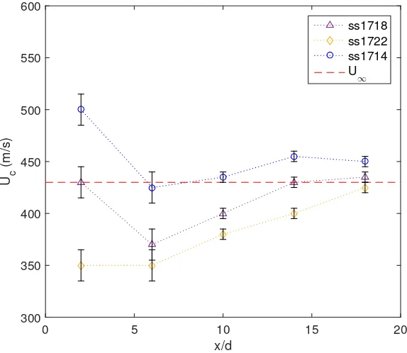
Figure 3.3: Convective-velocity estimated using SICV. The uncertainty bars represent the typical standard deviation of the convective velocity measurements in the bin,±σ, at that location (cf. Fig. 2.7)

lower-Wjjet-fluid and higher soundspeed have higher convective velocities immediately downstream

of the jet orifice (x/d∼2) than the jets with lower soundspeed values. In all cases, the convected fluid quickly decelerates to a minimum (at approximatelyx/d= 6), then re-accelerates to values close to the freestream velocity. The higher convective velocity of the lower-Wj jets persists downstream

even after the jet-fluid re-accelerates, as shown in Fig. 3.3.

The deceleration then re-acceleration of the jet fluid can be explained by the interaction of the jet with the crossflow just downstream of the bow shock. The crossflow gas is shocked down to M∞,2 < 1 by the near-normal bow shock ahead of the jet and re-accelerates downstream of the

shock to match the free stream. The under-expanded jet exits the orifice at sonic conditions, and rapidly accelerates toMj,2>1. Santiago and Dutton (1997) report a jet Mach number of∼2 just

upstream of the Mach disk and barrel shock structure (cf. Fig. 1.1) for comparable conditions (sonic air jet in M∞ = 1.6 crossflow, J = 1.7). The jet fluid rapidly decelerates as it entrains (possibly) subsonic post-shock crossflow fluid, but re-accelerates as the crossflow accelerates to approach the pre-shock freestream velocity.

It is tempting, and typical (e.g., Gruber et al. 1997a), to interpret the mixing-delay length and convective-velocity observations in terms of the well-understood, experimentally validated expres-sions for entrainment, mixing, and convective velocity of planar shear layers (reviewed in Dimotakis 1991). The convective velocity,Uc,SL, at thex/d= 2 location, in fact, is close to that predicted for

an incompressible planar shear layer formed between a (hypothetical) sonic stream of (Ar+He) jet fluid, and aM = 1.5 stream of (N2) crossflow fluid, at conditions typical of those in the experiments

considered here, i.e.,

Uc,SL

U1 '

1 +rSLs1/2

1 +s1/2 , (3.1)

whereU1 is the high-speed stream velocity, andrSLandsare the low-to-high speed stream velocity

and density ratios, as shown in Fig. 3.4 (top right).

However, the predicted incompressible shear-layer growth rate (Dimotakis et al. 1984),

δ

x(rSL, s)'Cδ

(1−rSL)(1 +s1/2)

2(1 +s1/2_r SL)

h

1− (1−s

1/2_{)/(1 +s}1/2₎

1 + 2.9(1 +rSL)/(1−rSL) i

whereδ, here, is the visible thickness, and empirically,Cδ'0.37, and the predicted mixing transition

region, ltr,SL, i.e., the predicted region at which the Reynolds number based on the shear-layer

thickness (δ) reaches ≈104 _{(Konrad 1977, Dimotakis 1991, 2000), in such a planar shear layer do}

not account for the TJISCF behavior observed in the present experiments.

X He

0 0.2 0.4 0.6 0.8 1

U 2 /U 1 0.5 0.6 0.7 0.8 0.9 1 X_He

0 0.2 0.4 0.6 0.8 1

m/s 300 350 400 450 500 550 600 U c,SL ss1722 ss1718 ss1714 X_He

0 0.2 0.4 0.6 0.8 1

( δ /x) SL 0 0.05 0.1 0.15 X_He

0 0.2 0.4 0.6 0.8 1

l tr,SL /d j 0 5 10 15 20

Figure 3.4: Shear-layer velocity ratio (top left), convective velocity with measured TJISCF near-jet convective velocity (top right), growth rate (bottom left), start of mixing transition (Reδ >104,

Konrad 1977, Dimotakis 1991, 2000) in jet diameters, fordj=0.2 in. (bottom right)

3.4, bottom left), and would not transition to the Re > 104 _{turbulent mixing regime at all (Fig.}

3.4, bottom right). These predictions do not agree with available experimental data, indicating that planar shear-layer relations do not apply to the TJISCF.

While sheared regions are certainly present at the interface between the leading edge of the jet and the post-shock crossflow, for example, fluid streams that form the mixing region are not uniform or well characterized. Moreover, the toluene PLIF images of Gamba et al. (2015) show that the jet leading-edge mixing-region structure is different than that of a planar shear layer. Instead of deconstructing the TJISCF into smaller elements, it may be better to interpret the TJISCF as a whole and focus on its response to global parameters. An important global parameter is the jet Reynolds number, whose influence is discussed in the following section.

3.2

Jet-diameter effects

Most properties of a transverse jet in crossflow are reported to scale with jet diameter. In particular, both weak-jet (low-J) and strong-jet (high-J) expressions for jet penetration and trajectory are normalized by the jet diameter (cf. Section 1.1). The mean jet-fluid concentration decay as a result of dispersion and mixing along the jet axis of momentum-dominated (strong) jets in crossflow scales with jet diameter by mass and momentum conservation arguments (cf. Hasselbrink and Mungal 2001). Lin et al. (2010) measured time-averaged jet-fluid concentration using Raman scattering in a weak (J ∼2) jet in supersonic crossflow for two jet diameters and found that the mean jet-fluid concentration scales with jet diameter. Changing the jet diameter directly affects the Reynolds number, for example, that influences mixing and combustion processes across a range of scales. We pose the question: does mixing-delay length in a TJISCF scale with jet diameter, or have a different dependence on jet diameter and associated jet Reynolds number?

The Reynolds number plays a fundamental role in the transition to turbulent molecular mixing. In a planar shear layer, the transition to rapid molecular mixing (Konrad 1977, Koochesfahani and Dimotakis 1986) begins some distance downstream of the splitter plate, at a local Reynolds number based on the shear-layer thickness of approximately 104_{, that has since been identified as a}

far-field, self-similar regions of axisymmetric jets (Gilbrech 1991, Dimotakis 2000).

Mixing in the near field of a gas-phase axisymmetric jet, however, remains Reynolds-number dependent even beyond the mixing transition. Gilbrech performed fast-chemistry axisymmetric gas phase jet experiments using diluted F2 in NO, complementing the liquid phase jet measurements

of Dahm and Dimotakis (1987, 1990), and others. The liquid-phase data of Dahm and Dimotakis (1987) and gas-phase data of Gilbrech (1991) showed the flame length, Lf, has a dependence on

stoichiometry, φ, of the form

Lf

d∗ =Afφ+Bf . (3.3)

d∗_{is the jet source (or momentum) diameter (e.g., Dahm and Dimotakis 1987), and is a length scale} defined by the ratio of the mass flux to the (square root of) the momentum flux, with constants added that forced∗_tod

jif the ambient and jet densities are equal, and if the jet exit velocity profile

can be approximated by a top-hat, i.e.,

d∗ ₌ 2 ˙mj p

πρ∞Pj

, (3.4)

with ρ∞ the ambient density, and ˙mj andPjthe jet mass and momentum flux, respectively, i.e.,

˙

mj=ρjAjUj; Pj=ρjAjUj2 . (3.5)

Af is the stoichiometric coefficient that was used as a measure of mixing in the far-field, self-similar

region. Bf is the intercept, or ‘virtual mixing origin’. Gilbrech showed that for a given φ, Af

decreased with Reynolds number up to approximately 2×104_{, and did not change beyond that}

value. The ‘virtual mixing origin’, however, decreased through and beyond the transitional value of Re= 2×104_{and did not approach asymptotic behavior even at a Reynolds number of 150,000. As}

There are parallels between the ‘virtual mixing origin’ of an axisymmetric high-speed jet and the mixing-delay length observed in these TJISCF experiments that imply a possible mixing-delay length dependence on jet Reynolds number,

Rej= ρjUjdj

µj

. (3.6)

A set of experiments (see Table 3.2) was performed with two sets of identical jet- and crossflow-fluid compositions and pressures, but different jet-orifice diameters.

Table 3.2: Jet-diameter effects

Run Inj. U∞(m/s) Uj(m/s) J $ lm(x/d) Xj,dil

ss1719 RN2 427 686 0.96 4.11 5.1 He:0.9,N2:0.095

ss1714∗ _{RN1 427 686 0.97 4.11 6.2 He:0.9,N}

2:0.095

ss1720 RN2 427 277 0.95 0.66 4.2 Ar:0.995

ss1722∗ _{RN1 427 277 0.98 0.66 5.1 Ar:0.995}

∗_{cf. Table 3.1}

The results help examine the effects of jet diameter and associated jet Reynolds number (Rej)

on the reacting flowfield, and in particular, help determine whether the mixing-delay length has an Rejdependence.

Figure 3.5 shows chemiluminescence images of lower-Wj(He+N2, ss1714, ss1719) and higher-Wj

(Ar, ss1722, ss1720) jets with dimensions scaled by the jet diameter, wheredjis either 0.508 cm (0.20

in.), or 0.635 cm (0.25 in.). While jet penetration is also observed here to scale with jet diameter, as expected and reported in the literature (e.g., Lin et al. 2010), chemiluminescence measurements show that jets with a larger diameter,dj, mix, react and emit chemiluminescence earlier, i.e., further

x/d

-4 -2 0 2 4 6 8 10 12

y/d -1 0 1 2 3 4 5

d_j=0.20" W_j=7

x/d

-4 -2 0 2 4 6 8 10 12

y/d -1 0 1 2 3 4 5

d_j=0.25" W_j=7

x/d

-4 -2 0 2 4 6 8 10 12

y/d -1 0 1 2 3 4 5

d_j=0.20" W_j=40

x/d

-4 -2 0 2 4 6 8 10 12

y/d -1 0 1 2 3 4 5

d_j=0.25" W_j=40

Figure 3.5: From top to bottom, chemiluminescence images from $= 4.11 (He+N2 jet fluid) Runs

ss1714,dj= 0.20 in. (top) and ss1719,dj= 0.25 in. (center top), from$= 0.66 (Ar jet fluid) Runs

Normalizing the mixing-delay length by the physical jet diameter does not collapse the data (cf. Fig. 3.6). Molecular mixing and reaction occur some dist