Manuscript received March 6, 2017; revised March 23, 2017. This work was supported in part by Electromagnetic Remote Sensing (EMRS) Defense Technology Centre, established by the UK Ministry of Defense and University of Technology MARA, Malaysia.
N. A. Zakaria is with the Faculty of Electrical Engineering University of Technology MARA, Shah Alam, Selangor, Malaysia (e-mail: [email protected]).
M. Cherniakov, M. Gashinova, V. Sizov are from School of Electronic, Electrical and Computer Engineering, University of Birmingham, Birmingham, United Kingdom (email: [email protected]).
N. A. Zakaria, M. Cherniakov, M. Gashinova and V. Sizov
Clutter Analysis for Forward Scatter Micro-Sensors
Abstract—Analysis on the clutter characteristics are carried out to investigate the effect of vegetation clutter for ground-based Forward Scatter Radar. Experimental and statistical analysis are presented which involves measured and simulated clutter analysis. The results from the analysis are then compared with different operating frequencies and clutter strengths.
Index Terms— vegetation, clutter, FSR, VHF/UHF, radar
I. INTRODUCTION
Forward Scattering Radar (FSR) can be categorized as a bistatic radar when scattering angle is near 0 or, as the bistatic angle approaches 180° [1,2]. FSR system provides an efficient approach for detection of so called "difficult" targets which can be characterized either by low Forward Scatter Cross-Section (FS CS) or low speed. The only peculiarity of FSR is the absence of range resolution and the clutter can be easily picked up from the large area illuminated by transmitter and receiver antennas. This makes the clutter issue more critical in comparison with monostatic radars [3].
The performance of the FSR depends on signal-to-clutter ratio and on specific characteristics of clutters such as caused by foliage or wind [4, 5]. If the area is surrounded by the foliage or vegetation, the target signal can be masked which can reduce the radar system performance.
In order to estimate the performance of FSR under variety of environmental conditions, kinds of targets and processing algorithms involved, general analysis of Doppler target returns, interference signals, noise and clutters and perform computer simulation of possible FSR scenarios or, in other words, to develop a so called "synthetic environment " were implemented.
Synthetic Environment (SE) is a simulation environment based on using both modelled and measured data enabling estimation and analysis of radar system performance. High level of stationary and non-stationary clutter is one of crucial problem in radar detection [6]. Development of SE for analysis of Forward Scattering Radar Network performance in complex environment may therefore
become important simulation tool for engineers and end users. Repetitive experiments in computer internal timescale can be generated with SE. So, no more long time data generation using a real data measurement experiment.
The concept of Forward Scatter Micro-sensors Radar network for situational awareness in ground operation was explained in detail in [7]. This type of radar network is used in this research due to its robustness, easy deployment and low maintenance [7-9]. The network consists of number of nodes separated by short-range transmitter/receiver pairs (micro-sensors), operating in forward scatter configuration intended for the detection and/or recognition of moving ground targets such as personnel and vehicles entering into protected area and crossing the radar node's baselines. The micro-sensors are free drop from UAV which can be spread over the area of interest with random positions and utilizes continuous wave operation [10].
In this paper, the empirical study of ground clutter caused by vegetation that can affect the development of clutter in FSR is presented. This include several measurements to determine and analyzed the characteristics of ground based clutter. Then, the results are used to generate the simulated clutter-like signal. Hence, both measurement and simulated results are compared which can be used for SE generation in future.
II. EXPERIMENTAL PROCEDURES
There are a lot of work has been done to analyze the effect of clutter in Forward Scattering Radar (FSR) network. In this research, FSR network is using bistatic radar system configuration where the transmitter and receiver are separated within a distance called as baseline (BL). When the transmitter or receiver is placed in certain position in the surrounding area full with vegetation and foliage that grows on or near the baseline, it will add to the target signal and sometimes can even mask it which makes signal detection difficult.
The analysis on clutter in this research is based on statistical approaches on different environments varying from flat surface to dense wood. Furthermore, multiple measurements are carried out in each landscape with different weather conditions and wind speeds. Numbers of clutter signal data were recorded to analyze the characteristics of recorded clutter from various landscapes.
The measurement is using Forward Scatter Micro-sensors radar network system with multi-frequency transmitter and receiver. Omnidirectional antennas are used with the operating frequencies in VHF/UHF (64, 135, 173 and 434 MHz). The baseline distances used are varied from 50 m to 200 m. Figure 1 shows the measurement set-up.
Figure 1: Measurement set-up
For this analysis, long term measurement has been carried out in Horton Grange, Edgbaston, University of Birmingham (Figure 2). Out of all measurement test sites, Horton Grange is chosen due to its complex environment. It has a flat area with different kinds of vegetation such as large and small trees, bushes which is dense enough to create different scale (low, medium, strong and very strong) of vegetation clutter. This is an ideal place for vegetation clutter measurement.
The experiments are focused on the analysis of clutter signal and clutter characteristics. This measurement was done in the same FSR position to examine the dependency of clutter from windy conditions and observed for a long period of time (few days) to collect clutter at different weather conditions. With long term monitoring of selected areas accompanied by video surveillance, it will provide better understanding of the system functionality.
The received data signals from the measurements are compared with the video data. This is just to specify the system performance for 24 hours running experiments in real environment.
Figure 2: Long term measurement position in Horton Grange
III. CLUTTER ANALYSIS
The unwanted reflections from a vegetation creates noise-like signals that received by the receiver are what we called as clutter. The FSR network system is not robust to clutter.
absence of range resolution will cause the clutter pick up from a large area around the sensors. The omnidirectional antennas that are used as sensors also contribute strong clutter collections.
Vegetation and foliage are the main influence of clutter, especially in the presence of wind. Foliage such as branches and leaves from trees will sway in one fixed position. This swaying foliage under windy condition creates additional noise in Doppler frequency band [9].
A. Clutter Analysis Measurement
[image:2.595.69.277.541.690.2]Clutter signal is a non-stationary signal that received by the receiver. Based on the analysis, the main influence to clutter build up in ground-based radar is the wind speed as compared to others. This introduces noises that are considered as clutter that will create Doppler effect and can be detected by the receiver. Thus, the wind speed in this research are categorized into four conditions; low, medium, strong and very strong as stated in Table 1.
Table 1: Wind condition observed during the tests Wind Condition Average Wind Speed (km/h)
Low <10
Medium 10 – 20
Strong 20 – 30
Very strong (gale) >30
Large numbers of clutter signals were recorded with overall duration more than 5900 hours. Empirical analyses are carried out based on the recorded data. The example of typical non-stationary clutter recorded for 64, 135, 173 and 434 MHz frequencies are displayed in Figure 3 for 20 minutes during day time with low wind speed (less than 10 km/h). Compared with other test site, Horton Grange was observed as the strongest clutter due to complex vegetation in surrounding.
0 5 10 15
-0.1 -0.05 0 0.05 0.1
Time, min
A
m
pl
itude
,V
64 MHz
0 5 10 15
-0.1 -0.05 0 0.05 0.1
Time, min
A
m
pl
itude
,V
135 MHz
0 5 10 15
-0.1 -0.05 0 0.05 0.1
Time, min
A
m
pl
itud
e,
V
173 MHz
0 5 10 15
-0.1 -0.05 0 0.05 0.1
Time, min
A
m
plit
ud
e,
V
434 MHz
Figure 3: Low clutter signal for 64, 135, 173 and 434 MHz channel frequencies
Signals transmit (Pt)
4C TX
Signals received (Pr)
4C RX
RX position
[image:2.595.307.551.552.742.2]AWGN1,
σ1
LPF1,
f cut-off1
AWGN2,
σ2
AWGN3, σ3
noise floor
LPF2,
f cut-off2
Simulated clutter-like signal Adjustment
to dynamic range
+
Stage 1
Stage 2
Stage 3
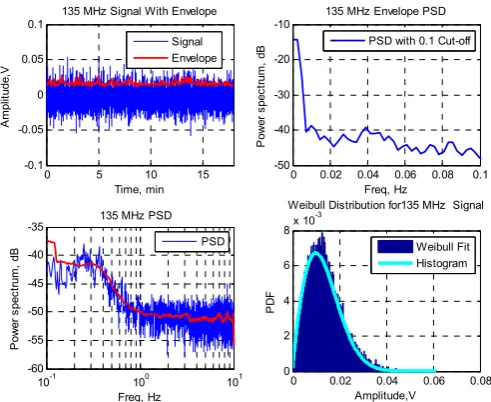
Each collected data will be processed and analyzed to determine the characteristic of clutter signal. Figure 4 displays the processed file for 64 MHz data with four types of output; Doppler signal with envelope, signal’s PSD, envelope PSD and Weibull distribution.
0 5 10 15
-0.1 -0.05 0 0.05
0.1 135 MHz Signal With Envelope
Time, min
A
m
pl
itude
,V
Signal Envelope
0 0.02 0.04 0.06 0.08 0.1
-50 -40 -30 -20
-10 135 MHz Envelope PSD
Freq, Hz
Po
w
er
s
pe
ctr
um
, d
B PSD with 0.1 Cut-off
10-1 100 101
-60 -55 -50 -45 -40
-35 135 MHz PSD
Freq, Hz
P
ow
er
s
pe
ctr
um
, d
B PSD
0 0.02 0.04 0.06 0.08
0 2 4 6 8x 10
-3
Weibull Distribution for135 MHz Signal
Amplitude,V
PD
F
[image:3.595.309.536.49.292.2]Weibull Fit Histogram
Figure 4: Analyzed data for 135 MHz channel for low clutter strength: Doppler signal, envelope PSD, signal PSD and Weibull distribution
[image:3.595.49.295.122.323.2] [image:3.595.327.534.513.615.2]All data taken from the measurement are summarized in Table 2. It has been processed and analyzed to find the value for the standard deviation, envelope’s minimum and maximum values, and Weibull’s shape factor for different clutter conditions. From the analysis, four different clutter conditions are identified such as low, medium, strong and very strong clutter. All the values for the different parameters are shown in Table 2. It shows that the clutter amplitude displayed in Figure 5, corresponds to the finding where the clutter amplitude increased parallel with the increment of clutter strengths.
Table 2 Measured clutter parameters for different clutter strengths
Freq (MHz)
Low Clutter Medium Clutter
STD
Envelope Weibull Fit STD
Envelope Weibull Fit
Min Max Min Max
64 0.0016 0.0024 0.0041 2 0.0145 0.0148 0.0405 1.95
135 0.0106 0.0095 0.0228 1.86 0.2518 0.0861 0.8593 1.71
173 0.0252 0.0118 0.0911 1.76 0.3068 0.0912 1.0618 1.64
434 0.0447 0.0137 0.152 1.67 0.3234 0.0773 1.3007 1.44
Freq (MHz)
Strong Clutter Very Strong Clutter
STD Envelope Weibull Fit STD Envelope Weibull Fit
Min Max Min Max
64 0.0247 0.0085 0.0939 1.75 0.03658 0.0173 0.2694 1.7
135 0.4471 0.1312 1.8141 1.67 0.6673 0.1544 2.7789 1.66
173 0.5536 0.143 2.4551 1.44 0.7259 0.1533 3.0868 1.41
434 0.6561 0.1634 3.2627 1.33 0.9493 0.0834 4.2691 1.19
Figure 5: Non-stationary clutter for all clutter conditions
B. Simulated Clutter Analysis
After the results on measured clutter are analyzed, the estimated parameter values such as standard deviation and envelope’s maximum and minimum values are then used to generate the clutter-like signal in order to have similar characteristics as the measured clutters with the spectrum up to 0.5 Hz and envelope spectrum up to 0.001-0.02 Hz characterized by higher power for higher frequency and having non-Gaussian distribution of amplitudes with some degree of similarity to a Weilbull distribution. The procedures of clutter generation are explained in detailed in [10]. Figure 6 shows the process to generate the clutter-like signal.
Figure 6: Vegetation clutter simulation model block diagram
All the output from the clutter generations are tabulated in Table 3 from low to very strong generated clutter signals. From the table, it can be concluded that the output of the generated signal have approximately similar trend with the measured signal. The output of the simulated signal can be seen in the next part of this paper.
-0 5 10 15
-0.1 -0.05 0 0.05 0.1
135 MHz
Time, min 0 5 10 15
-1 -0.5 0 0.5
1 135 MHz
Time, min
0 5 10 15
-2 -1 0 1
2 135 MHz
Time, min
0 5 10 15
-3 -2 -1 0 1 2
3 135 MHz
Time, min
Am
plitude,
V
Am
plitude,
V
Low Clutter Medium Clutter
[image:3.595.45.292.520.764.2]0 5 10 15 0
0.005 0.01 0.015 0.02 0.025
0.03 Low clutter strength
Time, min
A
mp
lit
ud
e,
V
A: Measured B: Simulated
0 5 10 15
0 0.2 0.4 0.6 0.8 1
Medium clutter strength
Time, min A: Measured B: Simulated
0 5 10 15
0 0.5 1 1.5 2
Strong clutter strength
Time, min
A
m
pl
itud
e,
V
A: Measured B: Simulated
0 5 10 15
0 0.5 1 1.5 2 2.5 3
Very strong clutter strength
Time, min A: Measured B: Simulated
0 0.01 0.02 0.03 0.04 0.05 0.06 0.07 0.08 0.09 0.1 -35
-30 -25 -20 -15 -10 -5
0 Measured PSD for 135 MHz
Freq, Hz
P
ow
er
sp
ectr
um
, d
B
A: Low B: Medium C: Strong D: Very strong
A B
D C
0 0.01 0.02 0.03 0.04 0.05 0.06 0.07 0.08 0.09 0.1 -35
-30 -25 -20 -15 -10 -5 0
Simulated PSD for 135 MHz
Freq, Hz
P
ow
er
sp
ec
tr
um
,
dB
A: Low B: Medium C: Strong D: Very strong
A B
C
[image:4.595.46.290.64.338.2]D
Table 3 Simulated clutter parameters for different clutter strengths
Freq (MHz)
Low Clutter Medium Clutter
STD
Envelope
Weibull Fit STD
Envelope
Weibull Fit
Min Max Min Max
64 0.0023 0.0019 0.0043 2 0.0187 0.0107 0.0471 1.97
135 0.0113 0.008 0.0239 1.95 0.2577 0.1045 0.6913 1.88
173 0.0334 0.0147 0.0764 1.84 0.3929 0.1138 1.1509 1.76
434 0.055 0.0156 0.1754 1.75 0.4487 0.0691 1.4127 1.66
Freq (MHz)
Strong Clutter Very Strong Clutter
STD
Envelope Weibull Fit STD
Envelope Weibull Fit
Min Max Min Max
64 0.0245 0.0118 0.0964 1.81 0.0967 0.0259 0.2643 1.77
135 0.6273 0.1667 1.8279 1.75 0.9131 0.126 2.4431 1.67
173 0.8472 0.1701 2.3507 1.68 1.0638 0.0898 3.5329 1.61
434 1.1008 0.1437 3.7959 1.6 1.4475 0.072 4.1419 1.57
C. Clutter Analysis for Different Clutter Strengths
The comparison between simulated and measured parameters shows very small differences for each frequency value. Bear in mind, the simulated clutter signal is based on the random generated signal. So, the exact clutter signal similar to measured signal cannot be generated.
[image:4.595.323.530.253.538.2]Figure 7 shows the clutter envelopes for both simulated and measured at 135 MHz frequency for 18 minutes measurement time. It can be seen clearly that the range of amplitudes and the trends of the signals are approximately the same for low, medium and strong clutter strength except for very strong clutter strength, where the maximum distribution of simulated clutter amplitude is slightly increased. While for measured clutter, the maximum amplitude for very strong clutter only reached 2.0 V a few times as compared to simulated signal. This is based on real measured data where the amplitude of the clutter can be unpredictable due to wind conditions.
Figure 7: 135 MHz measured and simulated clutter envelopes for different
The amplitude distribution of other frequencies such as 64 MHz, 173 MHz and 434 MHz also exhibit approximately similar trend for all clutter strengths for measured and simulated clutter signals.
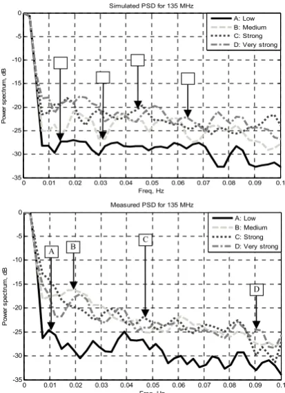
The clutter power spectral density shows in Figure 8 are the normalized power spectral density for simulated and measured clutter’s envelope for different clutter conditions. The trends of the envelope PSD are approximately the same for both simulated and measured graphs. It can be seen in the graphs below for 135 MHz and similar trends for other carrier frequencies. The spectrum of the clutter envelopes is about 0.01 to 0.02 Hz for all clutter strengths. This characteristic also resembles with other channel frequencies. This corresponds to 50 - 100 seconds of relative power homogeneity.
Figure 8: Simulated and measured clutter PSD for 135 MHz
D. Clutter Analysis for Different Frequencies
In this part, the comparison of simulated and measured clutter signals are based on different channel frequencies which varies from 64 MHz, 135 MHz, 173 MHz to 434 MHz. Only the lowest clutter strengths will be discussed as other clutter strengths such as medium, strong and very strong clutter strength also portrays similar trends of results.
Figure 9 and 10 shows the simulated and measured low clutter signals respectively. It can be seen in the figures that the clutter amplitude for both simulated and measured are within the same range of clutter voltage from 0.0041 V to 0.03 V, and the increased of clutter power from the lowest frequency of 64 MHz to the highest clutter power range of 434 MHz. This explains that the clutter power increased with the increase of frequency.
A
B
A
A A
B
[image:4.595.59.265.591.765.2]0 10 20 -0.1
-0.05 0 0.05 0.1
434 MHz
Time, min
0 10 20
-0.1 -0.05 0 0.05
0.1 173 MHz
Time, min
0 10 20
-0.1 -0.05 0 0.05
0.1 135 MHz
Time, min
0 10 20
-0.1 -0.05 0 0.05
0.1 64 MHz
Time, min
A
m
pl
itude
[image:5.595.49.288.48.235.2],V
Figure 9: Simulated low clutter for different frequency channels
0 5 10 15 -0.1
-0.05 0 0.05
0.1 434 MHz
Time, min 0 5 10 15
-0.1 -0.05 0 0.05
0.1 173 MHz
Time, min 0 5 10 15
-0.1 -0.05 0 0.05 0.1
64 MHz
Time, min
A
m
pl
itud
e,
V
0 5 10 15 -0.1
-0.05 0 0.05
0.1 135 MHz
[image:5.595.49.291.156.232.2]Time, min
Figure 10: Measured low clutter for different frequency channels
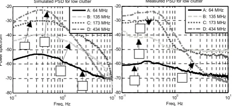
[image:5.595.49.286.350.458.2]Furthermore, the power spectral densities for simulated and measured low clutter are approximately within the same trends. The frequency channel that contributed the highest PSD is 434 MHz and the lowest is from 64 MHz channel frequency with the spectrum width of 10 dB power drop of 0.3 to 0.5 Hz for both simulated and measured clutters shown in Figure 11.
Figure 11: Simulated and measured low clutter PSD
IV. CONCLUSION
As a conclusion, it can be summarized from the results that the simulation and measured clutter signal are approximately the same for all characteristics that have been analyzed. This is shown clearly from the results that amplitude distribution exhibit Weibull distribution with the shape factor decreased with the increased of the frequency and clutter strength, the PSD trend and the clutter power increased with the increased of the frequencies.
Besides that, the spectrum of clutter is practically the same with the power dropped approximately around 0.005 Hz to 0.01 Hz and cutoff frequency of 0.1 Hz. The PSD slope drops approximately around 20 dB to 30 dB per decade for each channel. The spectrum width for different frequency channels which is defined by 10 dB power dropped are about 0.4 to 0.5 Hz.
Lastly, the results from this research can be used as a base to develop a synthetic environment for the analysis of Forward Scattering Radar Network performance in a
complex environment that can be used as a simulation tool for engineers.
ACKNOWLEDGMENT
This work reported in this paper was funded by the Electromagnetic Remote Sensing (EMRS) Defense Technology Centre, established by the UK Ministry of Defense and University of Technology MARA, Malaysia.
REFERENCES
[1] N. J. Willis and H. D. Griffiths, "Advances in Bistatic radar," Scientec Publisher, 2007.
[2] A. B. Blyakhman and I. A. Runova, "Forward scattering radiolocation bistatic RCS and target detection," in Radar Conference, 1999. The Record of the 1999 IEEE, 1999, pp. 203-208.
[3] M. Cherniakov, Ed., Bistatic Radar, Principles and Practice. John Wiley & Sons, 2007.
[4] V. Sizov, M. Gashinova, M. Antonio, and M. Cherniakov, "Signature Modelling and Coherent Target Detection for FSR Sensors," in IRS 2009, Hamburg Germany, 2009.
[5] H. R. Raemer, "Radar System Principle," CRC Press LLC, 1997.
[6] N. A. Zakaria, M. Gashinova, and M. Cherniakov, "Synthetic Environment for Forward Scattering Radar Detection," in Asia Pacific Defence and Security Technology Conference 2009, Kuala Lumpur, Malaysia, 2009.
[7] M. Antoniou, V. Sizov, H. Cheng, P. Jancovic, R. Abdullah, N. E. A. Rashid, and M. Cherniakov, "The concept of a forward scattering micro-sensors radar network for situational awareness," in Radar, 2008 International Conference on Radar, 2008, pp. 171-176.
[8] N. E. A. Rashid, Jancovic, P., M. Gashinova, M. Cherniakov, and V. Sizov, "The effect of clutter on the automatic target classification accuracy in FSR," in Radar Conference, 2010 IEEE, 2010, pp. 596-602.
[9] N. A. Zakaria, M. Cherniakov, M. Gashinova and V. Sizov "Empirical Clutter Analysis for Forward Scatter Micro-Sensors” 15th International Radar Symposium (IRS), 2014,pp. 1-4.
[10] M. Cherniakov, M. Gashinova, N. A. Zakaria and V. Sizov, "Empirical model of vegetation clutter in forward scatter radar micro-sensors " in Radar Conference 2010, Washington, DC, 2010, pp. 899-904.
10-1 100 101
-80 -70 -60 -50 -40 -30
-20 Measured PSD for low clutter
Freq, Hz
P
ow
er
spec
tr
um
,
dB
A: 64 MHz B: 135 MHz C: 173 MHz D: 434 MHz
10-1 100 101
-80 -70 -60 -50 -40 -30 -20
Freq, Hz
P
ow
er
spec
tr
um
Simulated PSD for low clutter A: 64 MHz B: 135 MHz C: 173 MHz D: 434 MHz
A
C D
B
A B C