Abstract—We propose the protocol of real-time quantum state estimation based on continuous weak measurement and compressed sensing (CS). We consider a pure ensemble of identical qubit spins which interacts with an optical mode and is measured continuously by homodyne detection. Assuming that the computing time is ignored, the state of the qubit ensemble can be estimated in real time. We verify the real-time estimation by simulation experiments on MATLAB. The evolution trajectories of the actual states and the corresponding estimated results are shown in Bloch sphere, and the influence of the parameters on the performance of the estimation results is analyzed. The experimental results show that when the system is under a constant applied magnetic field and the selected weak measure operator does not coincide with or be orthogonal to the Hamiltonian of the system, the state of the qubit ensemble can be accurately estimated in real time with only 2 consecutive measurements records.
Index Terms—compressed sensing, continuous weak measurement, quantum trajectory, real-time quantum state estimation
I. INTRODUCTION
UANTUM state tomography (QST), also called quantum state estimation or quantum state reconstruction, is one of the important contents in the research of quantum information processing and quantum control [1][2]. By estimating the state of the quantum system, people can effectively obtain the current information of the system and design the corresponding control scheme [3][4]. In order to fully estimate a quantum state, one needs to obtain the measurement values on a complete set of observables on the state. For an n-qubit quantum state, the number of complete observables is . In general, one needs to obtain the complete observation values by destructively measuring at least ensembles of identically prepared copies of the state. As a result, the number of measurements required for conventional QST increases exponentially as the number of qubits n increases, which brings great difficulties to the reconstruction of high-qubit quantum states.
2 2n 2n 4 d = × = n
2 d
Manuscript received December 8, 2017, revised January 10, 2018. This work was supported in part by the National Science Foundations of China under Grant No. 61573330 and No. 61720106009.
J. Yang, S. Cong and S. Kuang are with the Department of Automation, University of science and Technology of China, Hefei, 230027, China (corresponding author’s phone: 86-551-63600710; fax: 86-551-63603244; e-mail: [email protected]).
In some physical platforms, it is difficult to perform destructive strong measurements directly on the system. In order to obtain information of the target quantum system, people need to use a probe to associate with the quantum system and then measure the probe strongly. The information of the target quantum state can be inferred by the measurement records of the probe. If the interaction strength between the system and the probe is rather weak, this kind of measurement is called weak measurement [5] (Do not confuse this with another weak measurement concept related to the weak value [6]). Unlike the strong measurement that will completely destroy the state, weak measurement will only bring slight changes to the state and the impact to the system is also weak. Using weak measurements, one can measure a quantum ensemble and directly obtain the expectation value of an observable as the measurement record.
Since the weak measurement is not completely destructive, one can make continuous measurements of the quantum system with weak measurements. In continuous weak measurements, the observables are not orthogonal and the corresponding information between different observables overlaps, so the number of observables required to ensure complete information is usually greater than . Real-time quantum state estimation refers to the continuous state estimation of any moment based on the continuous weak measurement records of the quantum state. It is usually impossible to directly calculate the state of the quantum system by using non-orthogonal observables in continuous weak measurements. One can calculate the optimal result based on the measurement records using an estimator and an appropriate algorithm as the state estimation result. Real-time quantum state estimation is the basis of quantum feedback control, but there is yet no complete theoretical framework in this respect. Silberfarb et al. first proposed a quantum state estimation scheme and employed a continuous measurement protocol to perform QST on the seven-dimensional, F = 3 atomic hyperfine spin manifold, in an ensemble of cesium atoms [7]. Smith et al. achieved state-to-state quantum mapping performance estimation based on the continuous weak measurement, as well as the optimal control technology design and implementation [8]. And the quantum state of the spins undergoing the quantum chaotic dynamic of a nonlinear kicked top is measured based on the continuous weak measurement [9].
2 d
Compressed sensing (CS) provides a new solution to the problem of reducing the number of measurements in
Real-time Quantum State Estimation Based on
Continuous Weak Measurement and
Compressed Sensing
Jingbei Yang, Shuang Cong, and Sen Kuang
quantum state estimation [10]–[12]. CS claims that: if the rank of a state density matrix r is much smaller than its dimension d (r ), then the state density matrix can be reconstructed with only a small amount of randomly sampled measurement records. Gross proved that one can reconstruct the state density matrix with only
d
(
log)
O rd d measurement records when using the Pauli measurement operators [13]. CS can be applied to real-time quantum state estimation and improve the efficiency of calculation. Deutsch et al. first applied CS to the estimation of the states of a controlled quantum system under continuous weak measurements and realized the rapid reconstruction of the state of a 16-dimensional cesium atomic spin ensemble [14]. In this paper, we study the quantum state real-time estimation based on CS and the continuous weak measurement of one qubit spin ensemble. We verify the real-time estimation by simulation experiments on MATLAB using different control fields and different initial weak measurement operators. The evolution trajectory of the actual state and the corresponding estimated results in Bloch sphere are shown, and the influence of the parameters on the performance of the estimation results is analyzed.
The structure of this paper is organized as follows: In Sec. II, we give a detailed review of the principles of real-time quantum state estimation based on the continuous weak measurement and CS. In Sec. III, we verify the real-time estimation of the selected qubit spin ensemble by simulation experiments on MATLAB, and the influence of parameters, such as the control field and initial weak measurement operators, on the estimation performance is analyzed. Finally, a brief conclusion is given in Sec. VI.
II. PRINCIPLES OF REAL-TIME QUANTUM STATE ESTIMATION A. Quantum State Estimation
Quantum state estimation refers to the process of reconstructing the density matrix of the quantum state according to the measurement record and the corresponding measurement operators. In quantum mechanics, a measurement operator is a matrix that can reflect information or some mechanical quantities of the system, usually denoted by the operator M . The measurement of a d-dimensional quantum state
ρ
actually means measuring the expectation probabilities ofρ
projecting on a set of measurement operators . People can obtain one of the measurement valuesM ( )
j
M ρ corresponding to Mj by each measurement:
( ) ( )
j j
M ρ =tr ρM , j = 1, 2, … , d2 (1) In order to estimate the density matrix
ρ
, it is necessary for people to measure the expectation probabilities over multiple observables to obtain sufficient information. For an arbitrary quantum stateρ
of a d-dimensional Hilbert space, assume there is no priori information, it is generally necessary to measure on at least mutually orthogonal observables so as to accurately reconstruct2 1 d −
ρ
.Let M=
{
M1,M2,...Md2}
denote a set of completeobservables of
ρ
, including d2 orthogonal observablesj
M ( j = 1, 2, … , d2). M=
{
M1,M2,...Md2}
may beregarded as a set of basis corresponding to the Hilbert spaces. In this case, the density matrix
ρ
can be directly calculated by the following formula:2
1 1 d
i i
i
M M
d
ρ
=
=
∑
(2)When the selected set of observables is not complete, the measurement of
ρ
is called an informationally incomplete measurement. In this case,ρ
cannot be directly calculated by (2), but can only be calculated by using an optimization algorithm to calculate the closest estimation result under the existing conditions. In addition, the direct calculation of the density matrix using (2) is based on the assumption that the observables Mj are orthogonal to each other, whereas theobservables in actual tend to be non-orthogonal, such as generalized measurements, positive operator valued measurements (POVMs) and quantum weak measurements. And it is necessary to substitute the measurement records of the observables into an optimization algorithm to find the optimal estimation value through iterative calculation.
B. Quantum Weak Measurement
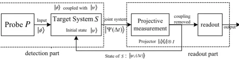
Quantum weak measurement is a method of measuring quantum state by using the weak coupling effect between the state and the probe [7]. It is usually used to measure quantum ensembles. Unlike the strong measurement that always causes instantaneous collapse of the target state, weak measurement is a non-transient measurement process, and the impact on the quantum system is weak. Weak measurement generally includes two parts: detection and readout. The process of weak measurement is shown in Figure 1, in which the left virtual box is for the detection part and the right virtual box is for the readout part. Weak measurement process introduces a probe which becomes coupled with the target ensemble for a short time for the detection part. Then the probe is strongly measured. Part of the information of the target S can be inferred with the measurement records of .
P S P
P
Target System
Probe measurementProjective readout
detection part readout part
( )t Ψ Δ
S Initial state
P
coupled with
joint system
φ ψ
Input
Projectori i⊗I
output coupling
removed
State of S:
φ ψ
( ) i t
[image:2.595.307.554.568.629.2]ψ Δ
Fig. 1. The process of weak measurement
When weakly measuring the target system S , the first thing is to prepare a probe . becomes coupled with resulting in a joint system
P P S
S⊗P. Suppose the initial state of the probe P is φ , and the initial state of the target system
is
S ρ0= ψ ψ . HS and HP are the Hamiltonian of
system S and P , respectively, and H =HP⊗HS is the
Hamiltonian of the joint system. The initial state of the coupled system is: Ψ = φ ⊗ψ . After the joint evolution of S and P for time Δt , the state Ψ
( )t U( )t
Ψ Δ = Δ Ψ , where U( )Δt is the joint evolution operator U( ) exp(Δ =t -iξΔtH/ )= , and ξ represents the interaction strength between system S and (the unit is 1/s ).
P
( )t
Ψ Δ is an entangled state composed of and which cannot be separately described with the states of
and . At time , a projective measurements
S P
S P Δt
X=
∑
i i i is performed on P , where i is the eigenstate of the system P , and i is the eigenvalue corresponding to i . After the projective measurement the entanglement between and disappears, and the weak measurement process is over. LetS P
( )
i
ψ
Δtdenote the state of S at time and the state of the joint system after the weak measurement is
t Δ
( ) (Δ )
i t i ψi t
Ψ Δ = ⊗ .
The weak measurement process can be regarded as a measurement operation on the system S, and the Kraus operator Mi is used to represent the weak measurement
operator. Therefore,
† 0
0 ( | )
i i i
M M
P i
ρ ρ
ρ
= (3) where ρi = ψi( )Δt ψi( )Δt is the state density matrix of S after the weak measurement. The weak measurement operator Mi is
( )
i
M = i ⊗ ⋅I U Δ ⋅t φ ⊗I (4) The weak measurement operators
{ }
Mi satisfy∑
iM Mi† i=1.0
( | )
P i ρ is the probability of measuring outcome : i
† †
0 0
( | ) Tr( i i ) i i
P i ρ = M Mρ = ψ M M ψ (5)
Let λ ξ= Δt denote the weak measurement strength, where both the interaction strength ξ and the evolution time of the joint system Δt are small values. Therefore λ is a small amount approaching 0 and Mi≈ iφ ⋅I which is
closed to 0 when i and φ are orthogonal or approximately orthogonal. Let Mi denote the weak
measurement value of Mi. Using the operators {Mi} and
the corresponding measurement values { Mi } , one can
estimate the pre-measurement state ρ0 and the post-measurement state ρi of the system S.
C. Continuous Weak Measurement and Quantum Trajectory
Continuous weak measurement means measuring the selected quantum system continuously using weak measurements. This is a dynamic process. One can obtain the information of the system based on the measurement records. Continuous weak measurement is usually used for the quantum feedback system. Based on the continuous measurement records, people can estimate the state of the system in real time and design a proper control law of the feedback.
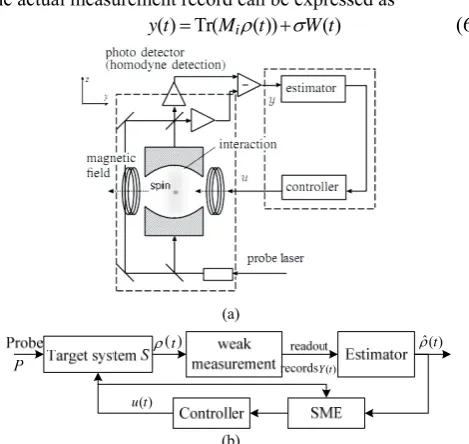
Taking the atomic ensemble ρ( )t in vacuum under a magnetic field as an example, the schematic of the experiment for continuous weak measurement and the
corresponding process structure diagram are shown in Fig. 2, in which the probe is a continuous laser beam. The initial state of the photon in the laser beam is φ , which coupled with the atomic ensemble ρ( )t resulting the output of the probe laser in the entanglement. The output probe is measured continuously by homodyne detection by the measurement operator X=
∑
i i i . Since the strength of weak measurement λ is very small, the back-action of the weak measurement is ignored. The weak measurement operators of this process are M dti( ) with different i, whererepresents the very short time interval required for the weak measurement and i is one of the possible measurement outputs. The probability of obtaining the output i on the
probe laser is . There exist shot
noises (SN) in the detection process, which will lead to a Gaussian distribution fluctuation in the actual measurement records. The measurement record can be modeled through a Weiner process W(t) with zero mean and unit variance and the actual measurement record can be expressed as
dt
†
( | ( )) Tr( i i ( ))
P i ρ t = M M ρ t
( ) Tr( i ( )) ( )
y t = Mρt +σW t (6)
(a)
( )
( )
Y t
ˆ( )t ρ
t
ρ
( ) u t
(b)
Fig. 2. (a) Schematic of the experiment under continuous weak measurement and (b) the process structure diagram of the schematic in (a) In the experiment shown as Fig. 2, the state ρ( )t cannot be completely estimated with only one measurement record of a certain moment t because the measurement operator related with only covers a small part of the information of
( )
y t
( )
y t
( )t
ρ . According to the principle of quantum tomography, a set of informationally complete measurement records is needed to fully estimate the density matrix of the state ρ( )t . Therefore, the system states must be estimated by using measurement records at different moments. The system dynamics is Markovian when ignoring the effects of weak measurements and shot noises. Assuming that all the parameters of the system except the state are known, if the state of a moment ρ( )tj can be estimated accurately, the
system dynamics trajectory with time can be established according to the known parameters. One can calculate the state of the system at any time with ρ( )tj and the dynamics
[image:3.595.311.546.304.526.2]due to the evolution [7]. The dynamics trajectory of a quantum system evolving over time is also known as the quantum trajectory, which is usually represented by the quantum state master equation (SME) [8].
The dynamics trajectory of the system in Schrödinger picture can be represented by the Lindblad master equation:
† † † ( ) [ ( )] 1 1 [ , ( )] ( ) ( ) 2 2 ( ) t t t i
H t L L t t L
L t L
L
ρ ρ
ρ ρ ρ
ρ = ⎛ = − − ⎜⎝ + +
∑
∑
= L ⎞ ⎟ ⎠ (7) where Lt[ ( )]ρ t is a super operator, and the operator Lrepresents the dissipation or decoherence caused by the measurement or the environment. The solution of (7) is
†
( )t t[ (0)] t (0) t
ρ
=Vρ
=Vρ
Vwhere is a super operator, and
(8)
t
V dVt dt=LVt t
s
. ,
(
exp 0 d)
t
t s
⇒V =T
∫
L , where T is the time-ordering operator. The state of the system changes with time because of the evolution. In order to facilitate the calculation, we transform system of Schrödinger picture into that of Heisenberg picture, where the measurement operator evolves continuously over time and the quantum state keep constant [7].If the super operator Lt[ ( )]ρ t is time-independent, then
the evolution equation of the measurement operator M ti( )
under Heisenberg picture is: † † † † ( ) [ ( )] 1 1 [ , ( )] ( ) ( ) 2 2 ( )
i t i
i
M t M t
i
H M t M t L L L LM t
L M t L = ⎛ = + ⎜ + ⎝ −
∑
∑
= L ⎞ ⎟ ⎠ (9)And the solution of (9) is: † ( ) [ (0)]
i t i
M t =V M
In particular, if the measurement is the ideal non-destructive measurement, the effect of measurement on the system is negligible and . When the system Hamiltonian does not change with time, the dynamics of the system under Schrödinger picture can be described by the Liouville-von Neumann equation:
(10)
0
L=
( )t i[ , ( )]H
ρ = −
= ρt
iHt
(11) The solution of (11) is:
( )t t[ (0)] exp(-iHt) (0)exp( )
ρ =V ρ = ρ
where the super operator . Ignoring the shot noises and the Weiner process in (6) is always 0, then the continuous weak measurement in Schrödinger picture is equivalent to the measurement of a constant quantum state
(12)
exp( )
t = -iHt
V
( )
W t
(0)
ρ with a continuously evolving measurement operator ( )
i
M t in Heisenberg picture. The evolving measurement operator M ti( ) in Heisenberg picture is:
†
( ) [ (0)] exp( ) exp( )
i t i i
M t =V M = iHt M -iHt
(13) And the corresponding measurement record is:
0
( ) Tr( i ( )) Tr( i( ) )
y t = Mρt = M t ρ
If the super operator
(14)
[ ( )]
t ρ t
L is time-dependent, then the evolving measurement operator M ti( ) in Heisenberg
picture is different from (13) because . In this case the operator
† †
t t
t D ≠ t D
V L L V
( )
i
M t is † † ( ) [ [ (0)]]
i t t i
M t =V L M
Due to the complexity of the calculation, it is difficult to give the solution of (15) directly. Deutsch et al. present a method of numerical computation with piecewise constant [7]: Suppose that Hamiltonian and super-operator are constant over any period of time , if is small enough, the measurement operator meets
(
(15)
i
t
L
i
t ti
] ( ]
0 i iM = M Vt , where .
1 ti
i i
t t+ =eLδ t
V V
It should be noted that, in Heisenberg picture, the measurement operators of different moments are a non-orthogonal. Since non-orthogonal operators are not independent of each other, the number of the operators for informationally complete is usually greater than d2.
D. Real-time Quantum State Estimation Based on Compressed Sensing
The theory of compressed sensing (CS) claims that if the density matrix ρ of a quantum state is a low-rank matrix, then the state density can be reconstructed with only
(
ln)
O dr d measurement of random observables by solving an optimization problem, where d and r are the dimension and rank of the density matrix ρ, respectively [13].
The reconstruction problem of density matrix ρ can be transformed into the following optimization problem:
*
min ρ s.t. y A= ⋅vec( )ρ , where ρ * is the nuclear-norm of ρ, vec( )⋅ represents the transformation from a matrix to a vector by stacking the matrix’s columns in order on the top of one another. The sampling matrix A is the matrix form of
the all the sampled observables Mi, and the sampling vector is the vector form of the corresponding observation values y
i
M . The above optimization problem of nuclear-norm is equivalent to the optimization problem of minimizing the 2-norm under the positive definite constraint:
2
minA⋅vec( )ρ −y s.t. Trρ=1, ρ≥0 (16) Equation (16) is also called nonnegative least squares optimization. Researchers have shown that the non-negative least squares optimization method also belongs to the CS optimization [19]. Two sufficient conditions for complete reconstruction of a matrix based on CS are: (1) the density matrix ρ is a low-rank matrix; (2) the sampling matrix A
satisfies the Restricted Isometry property (RIP) [13]. The vector and matrix can be expressed according to the current measurement configurations as:
y A
1 2
( , , ,
m
T
k k k
M M M
= ⋅⋅⋅
y ) (17)
1
2 vec( ) vec( )
vec( )
m
T k
T k
T k
M M
M
⎛ ⎞
⎜ ⎟
⎜ = ⎜
⎜ ⎟
⎜ ⎟
⎝ ⎠
A
#
⎟
⎟ (18)
where
i
k
M is an arbitrary measurement operator and
i
k
M is the corresponding measurement value.
It can be deduced according to CS that, if the sampling matrix formed by continuous weak measurement operators satisfies the RIP, then one can estimate the quantum state in real time with a small amount of time-evolving measurement operators
{
A
}
( )
i i
M t and corresponding measures records
{
y t( )i}
. Solving theoptimization problem (17) with an appropriate algorithm, people can obtain the reconstructed density matrix ρ.
III. SIMULATION EXPERIMENT AND ANALYSIS In this Section, we study the real-time state estimation of a qubit system by simulation experiments on MATLAB. We study the evolution trajectory and corresponding real-time estimated state trajectory of the controlled system. Through comparative experiments, the influence of external control field, control strength and weak observation observer on real-time state estimation is analyzed.
Consider a 1/2 spin particle ensemble ρ( )t as the object of real-time estimation, which is under z direction constant magnetic field Bz and x direction control magnetic field
cos
x
B = A φ. In Schrödinger picture, the initial state of the spin is ρ(0), and ρ( )t is the state at moment t.
A continuous weak measurement is applied to the system. The initial weak measurement operator is Mi. Ignore the
shot noises and assume the strength of weak measurement is 0
λ= . The evolution equation of the system is given by (11). The eigen-frequency of the spin ensemble ρ( )t in the magnetic field Bz is ω0=γBz , where γ is the spin-magnetic ratio of the particle ensemble, and Ω =γA is the Rabi frequency of the system Ω ∈\.
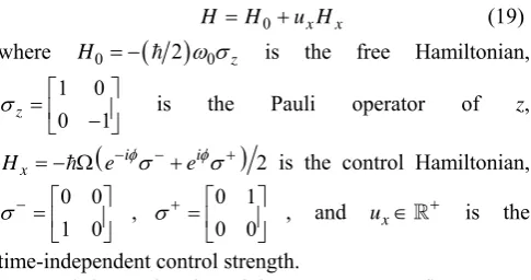
The Hamiltonian of ρ( )t is: 0 x x
H =H +u H
(19)
where H0= −
( )
= 2 ω σ0 z is the free Hamiltonian, is the Pauli operator of z,1 0
0 1
z
σ = ⎢⎡
−
⎣ ⎦
⎤ ⎥
)
(
i i 2x
H = − Ω= e−φσ−+eφσ+ is the control Hamiltonian,
, , and is the
time-independent control strength.
0 0 1 0
σ−= ⎢⎡ ⎤
⎥
⎣ ⎦
0 1 0 0 σ+ = ⎢⎡
⎣ ⎦
⎤
⎥ ux∈\+
In real-time estimation of the state ρ( )t , we first convert to Heisenberg picture. The estimated state is constant at this time and the measurement operator evolving over time is as Equation (13). Assume that the moment of continuous weak measurements are tj and the interval between two adjacent
moments is Δt.
The y t( )j are recorded from 0 moment. After each weak
measurement, substitute the recorded y t( )j
and corresponding
{
M ti( )j}
into (17) and (18) to get the real-time sampling vector and sampling matrix A . We use least-square algorithm to solve the optimization problem (16), and the optimal solutiony
(0)
ρ is the estimation of ρ(0). After obtaining ρ(0), the state density matrix at the current moment in Schrödinger picture is calculated according to (12), and the result ρ( )tj is the real-time estimation of the
state.
In the experiments, the fidelity f is used to represent the effect of state estimation:
1 1
2 2
( ) Tr ( ) ( ) ( )
f t = ρ t ρ ρt t
(20)
where ρ( )t represents the actual density matrix, and
( )t
ρ is the corresponding real-time estimated density matrix.
We choose the initial state of the 1/2 spin system as (0) [3 4 3 4; 3 4 1 4]
ρ = − − , and the Bloch sphere
coordinate of ρ(0) is
(
3 2, 0, 1 2)
. Let 180 2 2.5 10
ω = Ω = ×
= , the initial phase of Control field is φ=0 and the interval of the weak measurements is
18 0
0.4* 2 1 10 4 a.u.
t ω − s
Δ = = = × ≈ . Assume that the
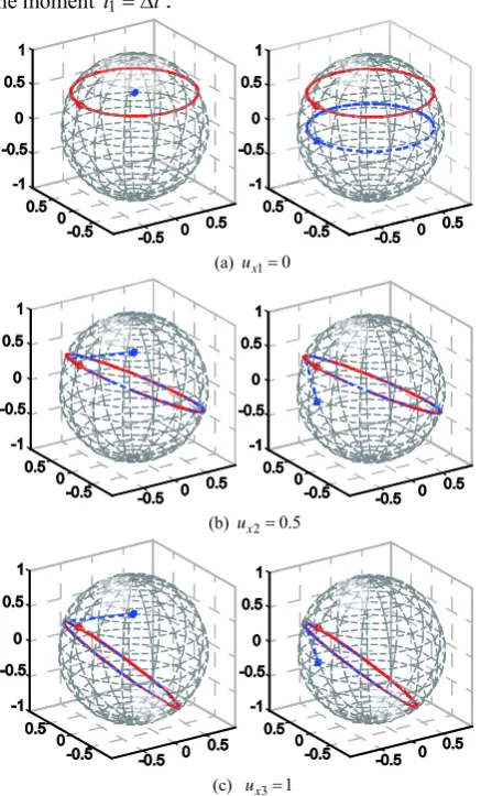
estimation time required is approximately 0. We choose three different control strength as ux1=0, ux2=0.5,
3 1
x
u = , and choose two kinds of initial weak measurement operators as 1 0
0 1 z z
M =σ = ⎢⎡ ⎤⎥ −
⎣ ⎦, for each
0 1 1 0
x x M =σ = ⎢⎡
⎣ ⎦
⎤ ⎥
control strength. Figure 3 shows the evolution trajectories of the actual state ρ( )t and the real-time estimation state
( )t
ρ in the Bloch sphere under different parameters, where the red solid line corresponds to the actual state, the blue dotted line corresponds to the real-time estimation state, " " represents the position of the actual initial state ο ρ(0), and " " represents the initial of estimation state * ρ(0). In Fig. 3, (a) (b) (c), respectively, correspond to the control strength ux1=0, ux2=0.5, and ux3=1, and the left and right columns of Fig. 3, respectively, corresponding to the measurement operators Mz and Mx.
At time t=0 , the initial estimated state ρ(0) is
calculated only from once measurement on the initial actual state ρ(0). Since ρ(0) in Fig. 3 is constant, the initial estimated state ρ(0) of the same column in (a) (b) (c) are same, but of different column are different. The fidelities of
(0)
ρ corresponding to Mz and Mx are fz(0) 0.7906= ,
(0) 0.9354
x
f = , respectively. It can be seen from Fig. 3 (a)
that, when ux1=0 , the actual system is under free
evolution and its evolution trajectory is a circular motion on x−y plane. The estimation corresponding to Mz is a
[image:5.595.48.291.585.713.2]axis, and the estimation corresponding to Mx is a
projection of ρ( )t on the x−y plane with z=0 . However when ux2=0.5 and ux3=1 , the evolution trajectories of the actual state have certain angles between the x−y plane, and the trajectories of estimation become coincide with the actual state trajectories in a short time. The value of control strength does not affect the accuracy of estimation. Comparing the experimental results of Fig. 3 we can see that: in Fig. 3 (a), when the measurement operators
z
M and Mx are coincident with or orthogonal to the free
Hamiltonian, the real-time estimation cannot achieve accurate results. However, in Fig. 3 (b) and Fig. 3 (c), the measurement operators Mz and Mx are not coincident
with or orthogonal to the system Hamiltonian, and accurate real-time estimations of the quantum state can be obtained at the moment t1= Δt.
(a) ux1=0
(b) ux2=0.5
[image:6.595.61.280.260.622.2](c) ux3=1
Fig. 3. The evolution trajectories of the actual state ρ( )t and the real-time
estimation state ρ( )t in the Bloch sphere under different parameters.
These experimental results show that, if the initial measurement operator is coincident with or orthogonal to the system Hamiltonian, continuous measurement cannot measure sufficiently valid information of the system and cannot achieve accurate real-time estimation of the state. On the contrary, if the initial measurement operator is not coincident with or orthogonal to the system Hamiltonian, a successful real-time estimation of the quantum state can be achieved, and the state evolving over time can be accurately estimated with at most 2 consecutive measurements records.
IV. CONCLUSION
In this paper, the real-time quantum state estimation based on CS and continuous weakness measurement is studied. We give the principles and schemes of real-time quantum state estimation, and analyze the influence of parameters on the performance of the estimation results. We verify the real-time estimation by simulation experiments. The real-time estimation of a 1/2 spin quantum state is realized, and different control strength and different initial measurement operators are respectively selected for the experiments. The evolution trajectories of the actual states and the corresponding estimation states are shown in Bloch spheres by comparative experiments. The experimental results show that when the initial measurement operator is not coincident with or orthogonal to the system Hamiltonian, an real-time estimation of the 1/2 spin system based on continuous weak measurements and CS is feasible, and accurate real-time estimations can be obtained with at most 2 consecutive measurement records.
REFERENCES
[1] G. M. D’Ariano, M. G. A. Paris, and M. F. Sacchi. “Quantum tomographic methods,” Lecture Notes in Physics, vol. 649, pp. 7-58, 2004.
[2] D. D’Alessandro,“On quantum state observability and measurement,”
Journal of Physics A: Mathematical and General, vol. 36, no. 37, pp.
9721-9735, 2003.
[3] C. J. Bardeen, V. V. Yakovlev, K. R. Wilson, S. D. Carpenter, P. M. Weber and W. S. Warren, “Feedback quantum control of molecular electronic population transfer,” Chemical Physics Letters, vol. 280, no. 1, pp. 151-158, 1997.
[4] Q. Sun, I. Pelczer, G. Riviello, R. B. Wu and H. Rabitz, “Experimental observation of saddle points over the quantum control landscape of a two-spin system,” Phys. Rev. A, vol. 91, no. 4: 043412, 2015.
[5] O. Oreshkov, T. A. Brun, “Weak Measurements Are Universal,” Phys. Rev. Lett. vol. 95, no. 11: 110409, 2005.
[6] Y. Aharonov, D. Z. Albert and L.Vaidman. “How the result of a measurement of a component of the spin of a spin-1/2 particle can turn out to be 100,” Phys. Rev. Lett. vol. 60, no. 14: 1351–1354, 1988.
[7] A. Silberfarb, P. Jessen and I. H. Deutsch, “Quantum state reconstruction via continuous measurement,” Phys. Rev. Lett. vol.
95, no. 3: 030402, 2005.
[8] G. A. Smith, A. Silberfarb, I. H. Deutsch and P. S. Jessen, “Efficient quantum-state estimation by continuous weak measurement and dynamical control,” Phys. Rev. Lett. vol. 97, no. 18: 180403, 2006. [9] S. Chaudhury, A. Smith, B. E. Anderson, S. Ghose and P. S. Jessen,
“Quantum signatures of chaos in a kicked top,” Nature, vol. 461, no.
7265, pp. 768-771, 2009.
[10] E. J. Candès, J. Romberg and T. Tao, “Robust uncertainty principles: Exact signal reconstruction from highly incomplete frequency information,” IEEE Transactions on information theory, vol. 52, no. 2, pp. 489-509, 2006.
[11] K. Zheng, K. Li, and S. Cong. “A reconstruction algorithm for compressive quantum tomography using various measurement sets,”
Scientific Reports, vol. 6: 38497, 2016.
[12] K. Li, H. Zhang, S. Kuang, F. Meng, and S. Cong, “An Improved Robust ADMM Algorithm For Quantum State Tomography,”
Quantum Information Processing, vol.15, no.6, pp. 2343-2358, 2016. [13] D. Gross. “Recovering low-rank matrices from few coefficients in any
basis,” IEEE Transactions on Information Theory, vol. 57, no. 3, pp. 1548-1566, 2011.
[14] A. Smith, C. A. Riofrío, B. E. Anderson, H. Sosa-Martinez., I. H. Deutsch, and P.S. Jessen, “Quantum state tomography by continuous measurement and compressed sensing,” Phys. Rev. A, vol. 87, no. 3: