This article provides information on methods for determining the size of a gas region in liquids and describes a laboratory bench and a program designed to automatically search for bubbles at the photo. This article, also, shows the correlation between the acoustic and photographic methods of bubble size determination. During this study a special program was developed and tested on images from laboratory bench. The Minnaert`s equation was approved by data delivered from acoustic and photographical methods. By the end of the study, the conclusions about program`s quality and it`s future development were reached.
Index Terms—bubbles size definition, acoustic bubble size, photo bubble size, measurement stand, Minnaert`s equation improvement, python program language, sample code, machine learning.
I.
I
NTRODUCTIONMeasurement of bubble size distribution and void fraction is important in multi-phase flow applications that range from flows subject to cavitation occurrence [19] and industrial processing, to oceanographic and biological flows. For example, in oceanography, determining the size of a gas cavitation allows you to find gas "torches": clouds of bubbles rising in the water column. For this purpose, the echolocation method (frequencies of 10–40 KHz) was used. This method is very sensitive and is able to detect the smallest single bubbles in the water column that are difficult or even impossible to observe visually. The composition of those bubbles is generally methane (99.9%). Searching for methane emissions and estimating the gas flow carried by bubbles is one of the urgent tasks of remote acoustic monitoring of the ocean.
Several techniques have been used to-date to obtain such information. These techniques can be divided into optical methods (photography, holography, scattering, radiography, etc.), acoustical methods [1] (scattering, attenuation, dispersion, etc.) and others.
Manuscript received March 18, 2019.
Dr. M.V. Ivanov is with the Bauman Moscow State Technical University, Moscow, 105005 Russia (corresponding author phone +79153303469; e-mail: [email protected]).
S.A. Gavriliev is with the Bauman Moscow State Technical University, Moscow, 105005 Russia (e-mail: [email protected]).
J.M. Tyurina is with the Bauman Moscow State Technical University, Moscow, 105005 Russia (e-mail: [email protected]).
A. Yusipova is with the Bauman Moscow State Technical University, Moscow, 105005 Russia (e-mail: [email protected])..
M.D. Boldyrev is with the Bauman Moscow State Technical University, Moscow, 105005 Russia (e-mail: [email protected]).
This study was focused on the photographical method of bubble size determination [20] and on the automatization of the data processing, as well as getting actual bubble diameter from the photo.
Nowadays, determining the size of a bubble or another suspended particle in the water column is very important, since such methods as aeration and flotation (methods using gas energy) predominate in the water purification.
The water entering the flotation tank for treatment usually has certain impurities and a large number of suspended particles. In order to adequately clean the liquid from the pollutant, it is necessary to select the most effective size of a gas bubble that rises to the surface of the water to take a part of the pollutant and form the sludge on the surface.
The flotation process for the concentration of ores is a method by means of which one or more of the minerals in the ore (usually the valuable ones) are picked up by means of a liquid film and floated at the surface of a mass of fluid pulp. Here they are separated from the other minerals, which remain immersed in the body of the pulp. In general, the minerals which are floated are sulphides of metallic luster, but some other minerals of metallic luster such as graphite and some sulphides with adamantine luster, such as sphalerite and cinnabar, are amenable to treatment by the process.
To calculate the actual diameter and number of bubbles, it is necessary to take in view such factors, as change in pressure of the gas during it’s movement to the surface, as a result of pressure change, as well as the division and unification of bubbles during the process.
There can be an ineffective way: you can experimentally find the ideal parameters, trying different ways to adjust the flotation unit to a different flow and power, trying to get maximum efficiency, setting the effective bubble diameter for the new liquid every time before it’s purification, spending a lot of time on the entire experimental technique, but you can establish the maximum effective size of the gas with some device that will immediately show you the right way. Cause of simplifying the process and increasing efficiency, this paper discusses the method of acoustic determination of the size of the gas cavity, that is, the determination of bubble size using a hydrophone that removes the spectrum of noise emitted during gas movement in a liquid.
For the connection of the acoustic signal to a gas bubble in a liquid, there is the Minnaert equation:
Developing Photo Analyzing and Bubble
Processing Program on Python language
Mikhail V. Ivanov, Member, IAENG, Stepan A. Gavrilev, Member, IAENG, Julia M. Tyurina,
where a is the radius of the bubble, γ is the polytropic coefficient, pA is the ambient pressure, and ρ is the density of water.
This equation can also be used to find the resonant frequency of a bubble cloud with a as the radius of the cloud and ρ the difference between the density of water and the bulk density of the cloud. For a bubble in water at standard pressure this equation reduces to fa ≈ 3.26 m/s, where f is the resonant frequency of the bubble.
The importance of this work proves many other works. For example, in Passive acoustic bubble sizing in sparged systems, by R. Manasseh, R. F. LaFontaine, J. Davy, I. Shepherd, and Y.-G. Zhu, the possibility of determining the size of a bubble using the frequency of an acoustic signal is being considered [13, 14, 15, 16].
When the bubbles rise to the surface, their shape is being changed. This affects to the frequency. As the speed of the air flow increases, the rate of bubble formation also increases. The rate of formation of bubbles can be considered high if the bubbles begin to collide. Under these conditions, Minnaert's equation cannot be used.
In that work there was an experimental part, in which it was found that the acoustic method for determining bubble sizes could well be used in practice, but you should take in mind that when a bubble rises to the surface, the spectrum is distorted. Thus, it can be said that the spectrum can be associated with the bubble radius only at the moment of the bubble appearance, provided that corrections were made for changes in frequency. Thus, it becomes clear that the best method would be to collect spectra of single bubbles, and not to measure the total spectrum.
Also, there was reviewed the «Development of an acoustic instrument for bubble size distribution measurement», by Xiong-jun Wu and Georges L. Chahine.[12] This article describes spectrometer «ABS Acoustic Bubble Spectrometer», which allows to measure bubbles in liquids with high accuracy in the range starting from 10 mkm to 3mm.
Also, article describes the solution getting integral of distribution bubbles by spectrum diagram, from hydrophone. In experimental part there also were used two and three hydrophones on different depth from energy appearance point.
Bubbles were also fixed on the camera, for comparing the photographic size with that picked by the acoustic signal.
The work “Dynamics of the Distribution of Bubbles in Sizes in Acoustic Fieldsæ, by the author A. M. Agrest and G.N. Kuznetsov, considers translational motion under the action of a pressure gradient of a number of pulsating bubbles of various sizes uniformly distributed in space at the initial time. The change in the size distribution function of bubbles depending on time and space coordinates is determined.
The bubble distribution function by size and space changes irreversibly at each point of the liquid volume under the influence of pressure gradients in a non-uniform acoustic field. This means that under the action of ultrasound, the treatment of the liquid occurs, leading to a change in its cavitation parameters. Also, in the area of the antinode of pressure, as a result of the action of the sound field, the
number of bubbles concentrates, significantly exceeding the initial one.
There was obtained the equation [11]:
,
where S(r) — volume enclosed between surfaces
u(r, R) — bubble velocity dependent on bubble coordinate and radius,
G(R) — bubble concentration.
The equation can be used to describe changes in the concentration and distribution function of bubbles in a stationary non-uniform hydraulic field, as well as to determine the concentration of solid suspensions in a liquid medium, provided that there is a cause that creates a directional motion of solid particles.
II. GETTINGDATA
At the first step of data collection. the following stand was constructed. [2]
Fig.1 stand plan
It consists of compressor (1), pipes (2) to bubble producing aerator (3)(4). At different depth in the aquarium, there was putted three hydrophones (5). The hydrophones connected to the computer (7) using wires (6). Computer using special program runs fast fourier transform on hydrophone`s data getting water noise specter [3]. Using graphical data and Minnaert equations [4], that shows that the frequency of the acoustic signal is directly related to the bubble size, we can calculate real bubble size.
On the tripod near glass camera (8) was installed. With this camera we have been getting images during our experiment.
The experiment was conducted as follows: the compressor was turned on, the regulator in front of the aerator regulated the pressure of the air entering the aerator itself, thereby changing the size of the gas bubbles. After that, we took photo shots and took a chart from three hydrophones.
Later, this data set was used for developing program. Also, during the experiment, there was acoustic specter obtained from hydrophones. The analysis of the data was carried out and charts were built. Also the transformations were made according to Minnaert's equation.
For each experiment, there were a series of photographs and acoustic samples taken due to level down the possibility of error and reduce one.
III.
PROGRAMDEVELOPMENTFor images processing was decided to use python developing language [5]. This language was chosen by following reasons:
1. Python is very easy for starting;
2. It has lots of libraries for working with images;
3. Any other developer can continue working with program, because python has very readable syntax;
For working with images there are two biggest libraries for python: PIL [6] and openCV [7]. For using PIL there are several reservations such as developer must know exactly what he is looking for at image. PIL requires to know dots array of the sub-image. Couse, we don’t have this data for searching, we decided to use openCV.
OpenCV was started at Intel in 1999 by Gary Bradsky, and the first release came out in 2000. Vadim Pisarevsky joined Gary Bradsky to manage Intel’s Russian software OpenCV team. In 2005, OpenCV was used on Stanley, the vehicle that won the 2005 DARPA Grand Challenge. Later, its active development continued under the support of Willow Garage with Gary Bradsky and Vadim Pisarevsky leading the project. OpenCV now supports a multitude of algorithms related to Computer Vision and Machine Learning and is expanding day by day.
OpenCV supports a wide variety of programming languages such as C++, Python, Java, etc., and is available on different platforms including Windows, Linux, OS X, Android, and iOS. Interfaces for high-speed GPU operations based on CUDA and OpenCL are also under active development.
OpenCV-Python is the Python API for OpenCV, combining the best qualities of the OpenCV C++ API and the Python language.
Let’s look at sample code below:
1. import numpy as np
2. import cv2
The next step was reading image from directory. OpenCV provides api for doing this operation.
1. image = cv2.imread("example.jpg")
After it, we need to make some mappings with loaded image. At first — add sharpest, put gaussian blur [8] and convert image to gray one for raising contrast. After this we save generated image in project folder and go on
The second step is searching for contrast deltas on gray image. It is difficult task for any other language except Python, because it also provides api for this operation
1. edged = cv2.Canny(gray, 25, 140)
2. cv2.imwrite("edged.jpg", edged)
Third step is adding morphological map and saving new image.
1. closed = cv2.morphologyEx(edged, cv2.MORP H_CLOSE, kernel)
2. cv2.imwrite("closed.jpg", closed)
Morphological map allows us to smooth the gaps, that we have gotten in previous step [9]. Also, this map paint up free space between two parallels closed contours.
Finally, we use cycle for enumeration contours, calculation pixel area and generation new diameter of bubble with center in contour. We did this operation because bubble, while getting upper to surface transforms from round to oval one.
1. cont,hier=cv2.findContours(closed.copy(), cv2.RETR_EXTERNAL, cv2.CHAIN_APPROX_SIMP LE)
2. total = 0
3. for c in cont:
4. peri = cv2.arcLength(c, True)
5. area = abs(cv2.contourArea(c)); #cal
c square
6. approx = cv2.approxPolyDP(c, 0.02 * p eri, True) #close contours
7. if len(approx) > 5: #number of kinks
8. (x,y),radius = cv2.minEnclosingCi rcle(approx)
9. center = (int(x),int(y))
10. radius = int(sqrt(area/pi)) #real
radius
11. cv2.circle(image,center,radius,(0 ,255,0),2)
After all of this we get a series of transformations with founded bubbles on image
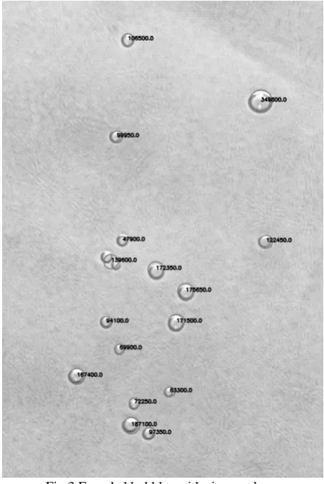
Fig.3 Founded bubbles with size mask Let`s have a detail look at the output image.
As we can see, there are a number of bubbles that were found very accurately. As a rule, such objects are in the most contrast part.
Also, it is clear that in the dark and non-contrast parts some bubbles were not found at all.
The bubbles, which were at different distances from the shooting plane, but layered on each other on image, for the program, turned into one bubble.
Also, it should be noted that the area values found are in pixels. To convert them into natural values, it is necessary to have a dimensional grid, and also to take in mind the curvature of the walls of the aquarium, the refraction of the liquid and the distance of the bubble's ascent line from the plane of the vessel wall.
IV. RESULTS
[image:4.595.323.524.180.338.2]As a result of getting data from hydrophones this graphical data was gotten:
Fig 3. Hidrophones graphs
Where horizontally the frequency of the sound in hertz is plotted, and vertically the volume in decibels.
Using Minaert’s equation, frequency values can be easily convert to the diameter of a bubble.
For doing this, the frequency value is inserted into the equation and the result is obtained. Based on the graph above, you can easily obtain a graph of the distribution of the size of the bubbles.
[image:4.595.47.284.659.760.2]As an output result of our program, we can also generate a graph of the size distribution of bubbles:
Fig 4. Program graph
The diagram shows the distribution of bubbles in the volume of liquid, which was able to photograph. Along the Y axis, we see the number of bubbles in dozens of pieces. The X axis represents the bubble area in mm.
As we can see, a correlation of peaks is seen in the results taken from the hydrophones and as a result of the distribution of the bubbles found. It means that our program works absolutely right.
In order to verify the efficiency of the equation and ensure that the data obtained by us above was not a mistake, we had repeated this experiment twice.
The new experiments confirmed the data gotten earlier: the program works, and the Minnaert`s equation is confirmed by the results taken.
V. CONCLUSION
The Minnaert`s equation`s applicability for liquid conditions was successfully confirmed.
There diagram of the data taken by the acoustic method was built. Afterwards, it’s correlation with the distribution data of the bubbles obtained by the photometric method was shown.
Thus, we can conclude that the task of determining the size of a bubble from a photograph is quite possible, with the following conditions adherence: the background of the image should be of the same type, the contrast should be of the same level. There should not be any suspended matter.
REFERENCES
[1] Leighton, T. (2012). The acoustic bubble. Academic press.
[2] Malmstrom, J. A., Beck, K. F., & Miles, S. D. (2003). U.S. Patent No. 6,531,708. Washington, DC: U.S. Patent and Trademark Office.
[3] Welch, P. (1967). The use of fast Fourier transform for the estimation of power spectra: a method based on time averaging over short, modified periodograms. IEEE Transactions on audio and electroacoustics, 15(2), 70-73.
[4] Devaud, M., Hocquet, T., Bacri, J. C., & Leroy, V. (2008). The Minnaert bubble: an acoustic approach. European Journal of Physics, 29(6), 1263.
[5] Van Rossum, G., & Drake, F. L. (2011). The python language reference manual. Network Theory Ltd.. [6] Umesh, P. (2012). Image Processing in Python. CSI
Communications, 23.
[7] Bradski, G., & Kaehler, A. (2008). Learning OpenCV: Computer vision with the OpenCV library. " O'Reilly Media, Inc.".
[8] Hummel, R. A., Kimia, B., & Zucker, S. W. (1987). Deblurring gaussian blur. Computer Vision, Graphics, and Image Processing, 38(1), 66-80.
[9] Vogt, P., Riitters, K. H., Estreguil, C., Kozak, J., Wade, T. G., & Wickham, J. D. (2007). Mapping spatial patterns with morphological image processing. Landscape ecology, 22(2), 171-177.
[10]Simonyan, K., & Zisserman, A. (2014). Very deep convolutional networks for large-scale image recognition. arXiv preprint arXiv:1409.1556.
[11]Manasseh, R., LaFontaine, R. F., Davy, J., Shepherd, I., & Zhu, Y. G. (2001). Passive acoustic bubble sizing in sparged systems. Experiments in Fluids, 30(6), 672-682.
[12]Wu, X. J., & Chahine, G. L. (2010). Development of an acoustic instrument for bubble size distribution measurement. Journal of Hydrodynamics, 22(1), 325-331.
[13]Christensen, M., & Thomassen, P. (2014). Experimental Determination of Bubble Size Distribution in a Water Column by Interferometric Particle Imaging and Telecentric Direct Image Method (Doctoral dissertation, Masters thesis Aalborg University).
[14]Devin Jr, C. (1959). Survey of thermal, radiation, and viscous damping of pulsating air bubbles in water. The Journal of the Acoustical Society of America, 31(12), 1654-1667.
[15]Crum, L. A. (1980). Measurements of the growth of air bubbles by rectified diffusion. The Journal of the Acoustical Society of America, 68(1), 203-211.
[16]Cui, J., Hamilton, M. F., Wilson, P. S., & Zabolotskaya, E. A. (2006). Bubble pulsations between parallel plates. The Journal of the Acoustical Society of America, 119(4), 2067-2072
[17]Ivanov, M. V., & Ksenofontov, B. S. (2014). Intensification of flotation treatment by exposure to vibration. Water Science and Technology, 69(7), 1434-1439.
[18]Ksenofontov, B. (2019, March). Multistage model of flotation process for water purification. In IOP Conference Series: Materials Science and Engineering (Vol. 492, No. 1, p. 012033). IOP Publishing.
[19]Dobrokhodov, K., & Petrov, A. (2019, March). Methodology of dynamic pumps testing on high-viscosity liquids. In IOP Conference Series: Materials Science and Engineering (Vol. 492, No. 1, p. 012016). IOP Publishing.
[20]Sarimollaoglu, M., Nedosekin, D. A., Menyaev, Y. A., Juratli, M. A., & Zharov, V. P. (2014). Nonlinear photoacoustic signal amplification from single targets in absorption background. Photoacoustics, 2(1), 1-11. [21]Ksenofontov, B., Senik, E., & Ivanov, M. (2019,