The vehicle routing problem and its intersection with cross-docking

2017

The vehicle routing problem and its intersection

with cross-docking

Juan David Cortes Ortiz Iowa State University

Follow this and additional works at:https://lib.dr.iastate.edu/etd

Part of theTransportation Commons

This Dissertation is brought to you for free and open access by the Iowa State University Capstones, Theses and Dissertations at Iowa State University Digital Repository. It has been accepted for inclusion in Graduate Theses and Dissertations by an authorized administrator of Iowa State University Digital Repository. For more information, please [email protected].

Recommended Citation

Cortes Ortiz, Juan David, "The vehicle routing problem and its intersection with cross-docking" (2017).Graduate Theses and Dissertations. 17170.

by

Juan David Cortés Ortiz

A dissertation submitted to the graduate faculty

in partial fulfillment of the requirements for the degree of

DOCTOR OF PHILOSOPHY

Major: Business and Technology (Supply Chain Management)

Program of Study Committee: Yoshinori Suzuki, Major Professor

Michael Robert Crum Anthony James Craig Kevin Paul Scheibe

Lizhi Wang

Iowa State University

Ames, Iowa

2017

TABLE OF CONTENTS

Page

LIST OF FIGURES ... iv

LIST OF TABLES ... v

ABSTRACT ... vi

CHAPTER 1: INTRODUCTION ... 1

CHAPTER 2: AN EXAMINATION OF THE INTERSECTION BETWEEN VEHICLE ROUTING AND CROSS-DOCKING ... 5

Introduction ... 5

Literature review ... 7

Intersection of the VRP with Cross-docking ... 13

A model for vehicle routing with shipment consolidation ... 16

Model definition... 17

The real value of VRPC ... 19

Transformation from VRPC to VRPSD ... 21

Preliminary experiments ... 23

Computational experiments ... 29

Results ... 32

Discussion ... 36

Conclusion ... 38

Final remarks ... 39

CHAPTER 3: A METAHEURISTIC FOR THE CAPACITATED VEHICLE ROUTING PROBLEM WITH MID-ROUTE SHIPMENT CONSOLIDATION ... 43

Introduction ... 43

Literature Review... 44

Computational experiments ... 53

Results ... 55

Conclusion ... 57

CHAPTER 4: INCREASED PERFORMANCE THROUGH THE VEHICLE ROUTING PROBLEM WITH SHIPMENT CONSOLIDATION AND TIME WINDOWS ... 60

Introduction ... 60

Literature Review... 62

Proposed model ... 63

Computational experiments ... 71

Results ... 73

Discussion ... 76

Conclusion ... 78

APPENDIX: ADDITIONAL MATERIAL ... 80

LIST OF FIGURES

Figure 1 - General flow of a cross-dock ... 11

Figure 2 5n3f-K with VRPSD... 27

Figure 3 5n3f-K with VRPC ... 27

Figure 4 6n2f-k with VRPSD ... 28

Figure 5 6n2f-k with VRPC ... 28

Figure 6 6n2f-k-Cluster with VRPSD... 28

Figure 7 6n2f-k-Cluster with VRPC ... 28

Figure 8 7n2f-k VRPSD... 29

Figure 9 7n2f-k VRPC ... 29

Figure 10 - Number of split deliveries (SD) in the VRPC vs. the VRPSD ... 35

Figure 11 - Number of nodes with mid-route shipment consolidation (XD) ... 36

Figure 12 - Average improvement of the VRPC vs. VRPSD by problem size ... 37

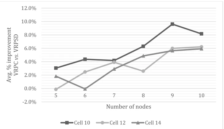
Figure 13 - Average savings through the VRPC vs. VRPSD in the top three cells of the experimental design ... 38

Figure 14 - Average performance gap of the objective value of the VRPCTW vs. VRPSDTW with the six-node problems ... 75

Figure 15 - Leaps variable selection plot ... 76

Figure 16 - Performance of the VRPCTW vs. VRPSDTW by levels of customer consolidation capability (Am) and network size for instances with shipment consolidation ... 77

LIST OF TABLES

Table 1 - Preliminary test instances for the VRPC ... 25

Table 2 - Optimal solution values for the VRPC vs. VRPSD ... 26

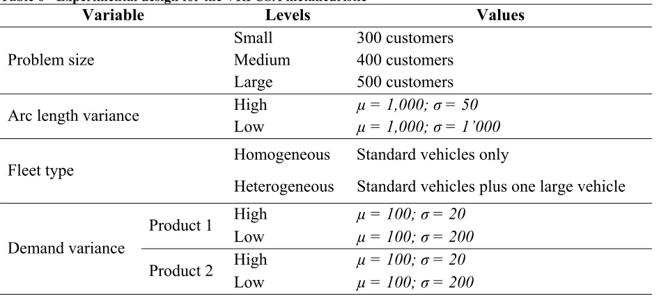
Table 3 - Experimental design for the VRPC ... 31

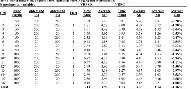
Table 4 - Performance of the proposed VRPC against the VRPSD, aggregated by problem size 33 Table 5 - Average computation time per model ... 36

Table 6 - Experimental design for the VRPCSA metaheuristic ... 54

Table 7 - Performance gap of the VRPC vs. VRPSD metaheuristics for 300 customers ... 55

Table 8 - Performance gap of the VRPC vs. VRPSD metaheuristics for 400 customers ... 56

Table 9 - Performance gap of the VRPC vs. VRPSD metaheuristics for 500 customers ... 56

Table 10 - Average results of the VRPCSA by problem size ... 57

Table 11 - Experimental Design for the VRPCTW ... 71

Table 12 - Top twelve best-performing cells of the VRPCTW vs. VRPSDTW with 5 nodes ... 73

Table 13 - Top twelve best-performing cells of the VRPCTW vs. VRPSDTW with 6 nodes ... 74

Table 14 - Performance gap of the VRPC vs. the VRPSD by problem size and cell. ... 80

Table 15 - Results of the VRPCTW vs. VRPSDTW with 5 nodes ... 83

ABSTRACT

To close a gap identified in the vehicle routing academic literature a theoretical link is

established between the Vehicle Routing Problem and Cross-Docking. A model for the vehicle

routing problem with shipment consolidation (VRPC), in which vehicles can consolidate cargo

among one another at a customer’s location, is presented. With shipment consolidation, vehicles

can deliver product to a customer, transfer product to another vehicle, or both. Three main

models are proposed: the vehicle routing problem with shipment consolidation (VRPC) which

improves routing performance by allowing vehicles to consolidate cargo at any customer site; a

metaheuristic to explore the effects of the VRPC over large-scale problems; and the Vehicle

Routing Problem with Shipment Consolidation and Time Windows (VRPCTW) to further study

the proposed concept under extended, more constrained circumstances. Computational

experiments are developed and solved to optimality where possible using OPL and Java in

conjunction with CPLEX and show that the proposed concept of shipment consolidation can

provide significant savings in objective function value when compared to previously published

CHAPTER 1: INTRODUCTION

After its first study was published (Dantzig & Ramser, 1959), the Vehicle Routing

Problem has continued to receive focused attention from scholars. Numerous variants and

methodologies to solve this NP-Hard combinatorial optimization problem have been proposed.

There still are many opportunities to further its current understanding. This problem has

captivated the attention of various academic fields and that of practitioners in various industries

that interact with logistics in one way or another. One largely important reason is the fact that

logistics comprises an important part of the country’s economy. The logistics component of

supply chain management accounts for well over one trillion of the United States GDP.

Sustaining a strong 60 percent of this amount, are trucking costs alone. Furthermore, in most of

the last decade these transportation costs have exhibited an average growth of 5.5 percent, and its

rates are already expected to be higher for 2017. In 2015 alone, motor carriers accounted for

almost a staggering 600 billion dollars of total U.S. business logistics costs. All other modes of

transportation (i.e. parcel, rail, air, water, and pipeline), if summed together, barely reach half

that amount. Motors carriers even stood atop total inventory carrying costs for the U.S. business

logistics industry, surpassing them by nearly 200 billion in 2015 (ATKearney & Penske, 2016).

However, transportation is not simply a monetary component of the economy. The

human component is vastly important. The U.S. Bureau of Labor Statistics has disclosed that the

estimate demand for truck drivers is closing in on 1.7 million persons (ATKearney & Penske,

2016). With average wage increases of merely 2 percent between 2010 and 2015, companies

must find incentives to keep driver turnover under control. An example is how some

publicly-traded firms show higher rates of increase in employee compensation than they do in total

morale and decrease costs associated with driver turnover in significant proportions (Suzuki,

Crum, & Pautsch, 2009).

Lastly, the impressive growth of B2C e-market has led various firms (e.g. Walmart,

Costco) to change their strategies and make significant investments in information technology

and mathematically-driven computer models to help leverage their operations in the benefit of all

stakeholders. Examples of these issues are answers to questions such as: how do I fulfill this

customer’s order? Do we ship to store? Ship directly to the customer? Do we use on-hand

inventory from a store nearby? Do we ship from a different store or warehouse further away?

These are not queries that can be easily solved by a single employee within a reasonable amount

of time. Furthermore, customers are asking for increased service levels exhibiting

close-to-flawless quality. Thus, it appears safe to say that efficient computer models are in an ever-high

demand.

Supply chain management and, more specifically, logistics must show that it can be a

major cornerstone in the creation of value-adding activities, not simply a capacity to move things

from a source to a customer. The industry and its representatives must converge in techniques

adequate to support value-creating activities throughout their supply chains. Examples of current

problems in transportation pertain to issues such as selecting a less efficient transportation mode,

expediting ordinary shipments, miscalculating truck arrival/travel times, among others. One way

to approach solutions to these inefficiencies is via better analytical models within the logistics

knowledge domain.

In logistics, a widely studied model is that of the Vehicle Routing Problem, along with its

special case, the Capacitated Vehicle Routing Problem (CVRP). Its objective is to minimize the

each customer is visited exactly once to deliver or collect a fixed demand, without exceeding the

capacity of vehicles. In a separate research stream, scholars have extensively studied

cross-docking operations. Findings suggest cross-docking can significantly reduce costs and

improve productivity (Soltani & Sadjadi, 2010). The objective of cross-docking is to consolidate

shipments with a common delivery destination in a specialized warehouse with the intent to

reduce transportation costs without sacrificing customer service.

Currently there is room to provide a new model that generalizes the CVRP with

cross-docking. There are three characteristics which are noteworthy. First, the evident requirement of

the CVRP stating that the items required by a customer must be placed on the same vehicle (no

multiple deliveries are allowed). This particular shortcoming was addressed by what is now

known as the CVRP with split-delivery (VRPSD). Second, the CVRP assumes that the fleet is

comprised by unrealistically standardized vehicles. Finally, the cross-docking literature is yet to

evaluate the effects of having vehicles transfer payload (commodities) throughout the network,

relaxing the necessity of having formal cross-docking warehouses at various locations.

This essay aims to unfold the benefits of the proposed model of shipment consolidation in

vehicle routing problems. With consolidation, vehicles can meet at any customer location and i)

partially or completely fulfill the customer’s demand, or ii) transfer commodities among one

another. The approach has the potential to bring significant savings to the objective function’s

value (e.g. miles driven, fuel cost, time spent). This investigation also seeks to shed light on

some of the condition under which the decision to consolidate shipments may be more

worthwhile. Sequential interviews with supply chain practitioners, representatives of large TL

and LTL transportation companies, were conducted to help determine some of the most delicate

model and study whether the proposed concept of shipment consolidation is feasible under more

realistic, constrained scenarios.

This document is organized as follows. First, a model for vehicle routing with shipment

consolidation is proposed and studied by solving small-customer instances to optimality. Second,

a metaheuristic is proposed to study the effects of the proposed concept on large problems.

Finally, a more complex model is proposed and it includes variables regarding time scheduling,

CHAPTER 2: AN EXAMINATION OF THE INTERSECTION BETWEEN VEHICLE

ROUTING AND CROSS-DOCKING

Introduction

Vehicle routing continues to receive attention from various stakeholders. Even though the

Great Recession allegedly ended in 2009, the logistics industry continued to receive its aftermath

for the following years. It was not until 2007 when the industry started to recover and shortly

thereafter observed surprising revenue levels in 2014, when it reached $1.45 trillion. Logistics

costs accounted for 8.5 percent of the United States GDP in 2012 totaling $1.33 trillion.

Furthermore, transportation and Third-party logistics providers (3PLs) are expecting sustained

growth throughout 2015 and 2016. Traditionally, the logistics and transportation industry is

divided in logistic services, air and express delivery, freight rail, maritime, and trucking. The

trucking industry alone accounted for a substantial $643 billion revenue stream in 2012, as per

the United States American Trucking Association. Trending technological advancements are

encouraging 3PLs to merge and increase their cloud-based service offerings to help leverage

partners’ performance. In addition, cross-docking and multimodal transportation are becoming

increasingly attractive, and supply chain software is becoming ubiquitous. Railway operations

are gaining all–time popularity rates and better ways to delivery products from a source to a

customer in the supply chain are more important than ever. This does not constitute a simple

trend and is unlikely to fade away. One key aspect to highlight is that, even though the logistics

industry experienced significant growth, such a hike was due to a volume increase rather than a

rate increase. This means that rates can become stagnant, which requires operations be carefully

streamlined and vast efforts be placed in continuously improving logistics processes. Academics

the threshold to provide better service rates without significant compromise in quality, cost,

delivery capabilities, and flexibility, among other competitive priorities. One way to address

these necessities is to account for product variety in vehicle routing and incorporating freight

classes in analytical models. The much suggested increased complexity in mathematical models

(Katok, 2011) will complicate their application but will simultaneously improve their value and

favorable impact on daily operations. With numerous studies accounting the nuances that supply

chain and logistics practitioners face in their business efforts, research can help increase business

performance from various perspectives while contributing to the epistemology of our fields.

To that regard, a model is proposed model herein to improve the efficiency of logistics

operations. It accounts for various elements used in an LTL shipment’s freight class and uses

these elements to optimize the way in which demand is delivered to customers. Specifically,

factors of density (volume and weight) along with liability (value) of shipped products are

accounted for and carefully implemented to maximize the usage of available fleet space and

thereby minimize routing cost. The proposed model for the vehicle routing problem with

shipment consolidation (VRPC) merges the literature in vehicle routing with that of

cross-docking to propose a novel alternative that improves solution quality. Such model allows

vehicles to transfer cargo among one another at any customer location (i.e. shipment

consolidation). Whether the problem entails a heterogeneous or homogeneous fleet, various

commodities, and several shipment factors or dimensions (hereinafter referred to as facets, e.g.

volume, weight, value) the proposed model is suitable to readily identify solutions that can

With the proposed model, supply chains can be designed to utilize shipment

consolidation and take advantage of said improvements in vehicle deployment, while offering

savings in aspects such as space utilization, labor–hours, vehicle maintenance, or fleet size.

TMS are becoming increasingly ubiquitous and are now at the forefront of supply chain

planning and design. These systems can yield substantive savings in transportation costs.

Furthermore, computer specifications have evolved to a point that allows a better integration of

information systems and intelligent optimization aiding in a firm’s decision-making capabilities,

supported by rigorous mathematical models. All these systems aligned with efficient models that

consider real-world constraints and variables to solve realistic problems under reasonable times

are a necessity. The proposed model can aid to carefully evaluate decision scenarios that in the

long term can improve logistics performance altogether.

Literature review

Vehicle routing problem

The Vehicle Routing Problem VRP has been studied extensively after its first publication

by Dantzig & Ramser (1959), along with many different exact and approximate methodologies

to solve it, such as branch-and-bound, cutting plane algorithms, heuristics, and metaheuristics

(Michel Gendreau, Guertin, Potvin, & Taillard, 1999; Michel Gendreau, Hertz, & Laporte, 1994;

Lysgaard, Letchford, & Eglese, 2004; Mitchell, 2002; Toth & Vigo, 2002a). It is a combinatorial

optimization problem that exerts strong practical relevance and carries considerable difficulty.

Essentially, the VRP is concerned with establishing an optimal route for an available vehicle

fleet such that each vehicle departs from a depot, serves a set of customers, and returns to the

depot. Each variant of the VRP will have various imposed constraints for said route construction.

only perform either), vehicle capacity, time windows to visit each customer, a homogeneous (or

heterogeneous) fleet of vehicles, stochastic or deterministic customer demands, split deliveries or

single-visits to each customer, and symmetric or asymmetric distances (traversing an arc in one

direction has a different cost than in the opposite direction).

The most studied version of the VRP is the Capacitated Vehicle Routing Problem

(CVRP) (Toth & Vigo, 2014). The CVRP is comprised by a central depot, a set of n customers,

and a cost matrix denoting the cost (generally length) of each pair of arcs. Each customer has a

nonnegative demand, and a finite fleet of identical vehicles, based at the depot and with finite

capacity Q, is available to serve the customer set. The objective is to find the optimal route such

that: each route starts and ends at the depot; each customer is visited exactly once; the total

demand of each route does not exceed Q; and the total routing cost is minimized (Cordeau,

Gendreau, Laporte, Potvin, & Semet, 2002). Other variations to the CVRP include delivery and

collection (e.g. Sankaran & Ubgade, 1994; Golden, Assad, & Wasil, 2001), in which some

customers require the delivery of goods and, conversely, others require the pickup of goods. An

example would be in the case of good distribution to retailers while performing reverse supply

chain operations to recover defective items from the market. The routes generally only perform

either of these two operations. A special case of the CVRP with delivery and collection is that in

which linehaul (delivery) and backhaul (collection) customers can coexist in the same route.

Under these settings, linehaul customers are served first to have an empty vehicle the moment in

which the first backhaul is done. Similarly, the particular case called the CVRP with mixed

deliveries and collections in which there are no difficulties associated with the loading and

unloading of the vehicle and thus linehauls need not be served before backhauls (e.g. Min, 1989;

traversed any capacity constraints are not violated. Another relevant case to the topic in question

is the CVRP with Split Delivery or VRPSD (e.g. Archetti, Speranza, & Hertz, 2006; Dror,

Laporte, & Trudeau, 1994; Dror & Trudeau, 1989; Frizzell & Giffin, 1995; Ho & Haugland,

2004). These problems are more specifically tailored to events in which the total demand of a

customer exceeds the capacity of the vehicle, and thus more than a single visit becomes is

imperative. In addition, the cost savings that can be obtained by partially delivering goods have

proven to be considerable. In this setting, a customer’s order can be fulfilled by different

vehicles, each carrying a portion of the total order.

Cross-docking

Companies such as UPS, Toyota, and Walmart attribute great part of their success to

efficient usage of cross-docking systems (Yu & Egbelu, 2008). Furthermore, with time-varying

changes in oil prices, cross-docking is gaining outstanding popularity. Motor carriers, third-party

logistics companies (3PLs) and shippers are incessantly facing difficult challenges to help

leverage partner firms’ performance. 3PLs are merging and increasing their cloud based service

offerings, cross docking and multi modal transportation are becoming increasingly attractive, and

supply chain software is turning ubiquitous.

Cross-docking is one way to decrease logistics costs and help leverage partners’

performance. It is defined as “receiving product from a supplier or manufacturer for several end

destinations and consolidating this product with other suppliers’ product for common final

delivery destinations” (Kinnear, 1997). It increases customer service performance and also

outperforms traditional warehousing in inventory investment, storage space, handling cost and

order cycle time, inventory movement, and cash flow (Kuo, 2013). Cross-docking consists of

If these five elements are cooperating in tandem, cross-docking activities can reduce costs and

improve productivity (Soltani & Sadjadi, 2010). However, unlike a DC, cross-docking facilities

(i.e. cross-docks) typically store items for small periods of time. In an ideal scenario a cross-dock

would have no inventory and picking operations would be negligible. However, this is

realistically difficult to attain because nearly-impossible coordination would be required (e.g. all

the orders of a single supplier might not arrive at the same time, thus temporary storage is

required until all the necessary goods are available). Customers are requiring specialized

products and services at an increasingly faster delivery rate. Shippers and Third-Party Logistics

(3PL) companies are making an effort to increase customer service while keeping costs stagnant.

All five basic functions of a DC will generally have room for improvement, especially in cases

with greater product flow. However, the less handling and storage that a DC has to perform, the

better the operational performance of such facility (Yu & Egbelu, 2008). Therefore, we can

conclude that storage and picking are generally the two most expensive tasks in both

cross-docking and DC operations.

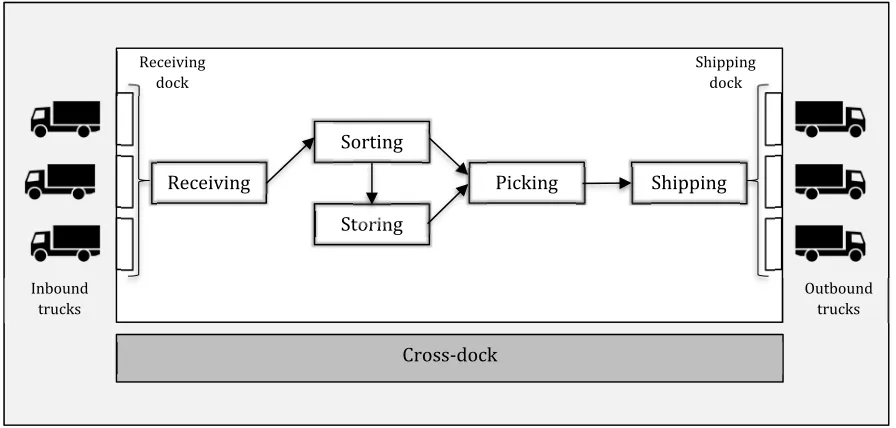
A traditional cross-dock typically operates as depicted in Figure 1. First, inbound trucks

arrive at a receiving dock where they can unload the items. These items can be of various sizes,

shapes, and packing. Ideally, trucks would experience no queue and they could be served

immediately. At this point, items are scanned and inspected, often weighed and labeled. Second,

they are placed on conveyer belts and sortation systems and subsequently taken to appropriate

sections based on their destinations. The most beneficial scenario is that in which there is no

need to temporarily store any items (Items can be immediately shipped out). However, if storage

is required then these items are set on hold in corresponding areas. Subsequently, when the time

Finally, the items are transferred to the appropriate location on the shipping docks, where they

are placed in outbound trucks and leave toward their next destination.

Figure 1 - General flow of a cross-dock

The objective of cross-docking is to serve as an order-consolidation warehouse where the

time items spend held in inventory is minimized. Naturally, the larger the firm the more likely it

is to have an increased inventory turnover and, by transitivity, lower cross–docking costs. The

cross-docking model can serve to consolidate product before last mile delivery and can be used

to switch transportation mode. It is expected that once a large-enough material handling volume

is attained, cross–docking becomes increasingly cumbersome and many challenges arise. There

are different technologies that can be set forth to improve its performance such as hardware (e.g.

RFID, GPS, barcode readers) and software (e.g. WMS, ERPs, custom software modules) but the

most important is the symmetry of information and secure yet fast and easy access to the

necessary information such that the parties involves can adequately plan the use of resources.

Cross–docks need be properly designed to adequately handle the product flow intended for it and

to do this, information transparency is of especial importance. The focus of conventional

Inbound trucks

Cross‐dock

Receiving Picking Shipping

Storing Sorting

Outbound trucks Shipping

dock Receiving

cross-docking models is the minimization of two main aspects of time: that which products

spend at the cross-dock and truck idle-time (unloading and loading). Typically, cross-docking

optimization models will assume that sorting and storage need not be optimized. Warehousing is

allowed but physical destinations inside the DC are commonly not established. Furthermore,

trucks generally stop once at either the receiving or the shipping dock when all of the relevant

cargo is either unloaded or loaded, and no revisits are allowed. Long-term (indefinite) storage is

not available. Temporary storage is possible but not ideal (the time-minimization objective

function would usually avoid these circumstances).

Even though considerable research has studied cross-docking and also vehicle routing

with loading constraints (Galbreth, Hill, & Handley, 2008; Michel Gendreau, Iori, Laporte, &

Martello, 2006; Kum Khiong Yang, Balakrishnan, & Chun Hung Cheng, 2010; Kuo, 2013;

Soltani & Sadjadi, 2010; Tarantilis, Zachariadis, & Kiranoudis, 2009; Vahdani & Zandieh, 2010;

Wei, Zhang, & Lim, 2014; Yu & Egbelu, 2008; Zhu, Qin, Lim, & Wang, 2012), very few

actually attempted to intersect both areas in a dynamic fashion. Wen et al. (2009) presented a

model labeled the Vehicle Routing Problem with Cross-Docking in which a set of homogeneous

vehicles is used to fulfill the orders of a customer set via a cross-dock. Their model uses a

cross-dock to consolidate orders while minimizing storage time and considering customers’ time

windows. Lee et al. (2006) published a similar model, in which multiple suppliers and customers

must be visited within an allotted time window. However, these publications are limited to a

single cross-dock at fixed coordinates.

The model presented in this study is the vehicle routing problem with shipment

consolidation (VRPC). This problem consists of single set of customers that require the delivery

with fixed capacity, whose tours start and end at a central depot. The VRPC has the particularity

that vehicles can consolidate cargo mid-route. To this end, vehicles can meet at any customer

location and i) partially or completely fulfill the customer’s demand, or ii) transfer cargo among

one another. This process will be hereinafter referred to as shipment consolidation. While this

approach relaxes the constraint that each customer can only be visited by one vehicle it has the

potential to considerably decrease the objective function’s value or total cost (e.g. miles

traveled).

Intersection of the VRP with Cross-docking

Scant studies have delved into the possibility of intersecting the CVRP with

cross-docking in a dynamic fashion. Most studies thus far have merged vehicle routing to and

from the cross-dock. However, they are both treated in the traditional fashion: vehicles move

cargo and the cross-dock transfers such cargo from one medium to another while the cross-dock

is at a fixed location. However, the proposed model attempts to evaluate a different approach and

thereby challenge the paradigm that a cross-dock need be a brick-and-mortar facility with fixed

coordinates. By relaxing these assumptions and allowing the model to propose dynamic

cross-docking points significant savings can be attained in the form of total distance covered,

which can further be generalized to reduced fuel consumption, fleet size, vehicle maintenance,

labor hours, among others.

To introduce the proposed model, a revision of the conventional Capacitated Vehicle

Routing Problem (CVRP) is appropriate. The CVRP consists of the schedule of sequential visits

to distribute goods from a single depot, denoted as zero (0), to a set of n nodes, typically referred

to as customers, such that N = {1, 2, …, n}. Each customer ∈ must has a specific demand,

delivered to the customers using a fleet of |K| homogeneous vehicles, such that

1, 2, … , | | , each of which has a standard capacity 0. The CVRP consists of routing each

vehicle to serve a subset of customers ⊆ to depart from the depot, visit each customer in S

once, and finally return to the depot. The CVRP can be set in either a directed or an undirected

graph depending on whether traversing an arc in a certain direction has a different cost than

traversing it in the opposite direction, or if such cost is equal regardless of the direction in which

it is traveled. We will focus in the more general case of the directed graph. The vertices or nodes

are the set 0 ∪ 0, 1, 2, … , and the arc set , ∈ : having cij be

the cost of traveling from node i to node j for , ∈ . The CVRP is thus uniquely defined by

the complete digraph , , , along with the vehicle fleet K of size |K| and the vehicle

capacity Q. A route or tour is a sequence , , , … , , where 0 in which

the subset , … , ⊆ of customers is visited. Each route r has a cost ∑ _,

associated. A route in which a) the capacity constraint ∶ ∑_∈ is not violated; and

b) each customer is visited only once (i.e. ∀ 1 ); is said to be a feasible

cluster ⊆ . A solution to the CVRP consists of |K| feasible routes, dictating the tours of |K|

available vehicles. A feasible solution will be the routes , , … , | | along with their

corresponding clusters , , … , _{| |} in which all the routes are feasible and the clusters form a

partition of N.

The CVRP becomes the solution of two simultaneous and interconnected tasks: i)

partitioning the set of customers N into feasible clusters , , … , _{| |}; and ii) routing each

vehicle ∈ along 0 ∪ . The complexity of the graph G is defined by | | 1 and

therefore we can conclude that it is of the form . The following is the basic formulation of

: ∉ , ∈ be the in-arcs of S and let , ∈ : ∈ , ∉ be the out-arcs of S.

Third, let , ∈ : , ∈ the subset of arcs connecting all vertices in S.

Furthermore, given a customer subset ⊆ , let be the minimum number of vehicle routes

needed to serve S. The lower bound of is given by the expression ⁄ . It is now

possible to proceed to establish a general form of the CVRP in a Mixed Integer Programming

(MIP) model with polynomial variables with respect to n = |N| and |K|.

(1.1)



  A (i,j) ij ij x c minimize subject to

(1.2) 1

) ( 



(1.3) 1

) ( 



(1.4) x K

j

j 





 (0) 0



N j 

(1.5) ( )

) ( ) , ( S x S j i ij





S N,S

(1.6)

x



 

0

,

1

The objective of the model (1.1) is the overall minimization of routing costs. The set of

constraints (1.2) and (1.3) guarantee that each customer vertex in a route is only connected to

two other vertices; in other words, that each customer is visited only once. Additionally, the set

of constraints (1.4) ensure that exactly |K| routes are constructed. These constraints can readily

be replaced with inequalities of the form “≤” if the fleet size is larger than needed or | | .

Next, constraints (1.5) are both capacity cut constraints and Subtour Elimination Constraints

tours not connected to the depot are also deprecated. Another approach is the MTZ formulation

(Miller, Tucker, & Zemlin, 1960), which replaces equations (1.4) and (1.5) and introduces the

additional variables , … , . These ui variables represent the cumulative demand

delivered by the vehicle after it arrives to customer ∈ . The MTZ formulation introduces the

following two sets of constraints as the SEC constraints and the capacity cut constraints,

respectively as follows:

(1.7)

u



u



Q



x



Q



q

(1.8)

q



u



Q

The advantage of the MTZ formulation is that it involves n2 _{+ n constraints and n}2 _{+ 2n}

variables. However, even though this formulation would have complexity, its linear

relaxation for the MIP model produces a significantly weaker lower bound (Toth & Vigo, 2014).

A model for vehicle routing with shipment consolidation

In this essay, mid-route commodity consolidation is presented as a form of cross-docking.

The objective corresponds with the goals of lean supply chain management: smaller volumes of

more visible inventories that are delivered faster and more frequently (Van Belle, Valckenaers,

& Cattrysse, 2012). The goal is therefore to capitalize on the capabilities of more frequent and

faster deliveries of cross-docking. The concept consists of turning every customer site into a bay

where a simple consolidation of shipments can be performed. The intended goal is to reduce total

distance covered by vehicles with less-than-truckload cargos. One of the main benefits of the

proposed model of VRPC is the lack of need for a specific location where cross-docking

operations are conducted. Consider the example in which two vehicles, k1 and k2, with

each other. Furthermore, assume that the total cargo of both vehicles can be consolidated in a

single truck (i.e. u1 + u2≤ Q). In this case, there should exist a point, not far from k1 and k2’s

locations, where either u1 is loaded onto u2, or conversely should that be more favorable. This

way, only one vehicle would continue traveling and the other could return to the depot.

Model definition

The problem is defined by G = (V, E), a complete graph where ∪ 0

0,1,2, … , is the set of nodes, and , | , ∈ is the set of edges joining each

pair of nodes. Let 1,2, … , | | be the set of customers and | | , and {0} be the central

depot. The distance of each arc , ∈ is denoted by dij. Let ∈ 1, 2, … , | | represent

the various commodities (products) customers require, and , , … , for ∈ , ∈

be the set of non-negative customer demands, with 0 ∀ ∈ . The fleet is comprised of

available vehicles ∈ 1,2, … , | | , where each vehicle k has a capacity of for each

facet ∈ 1, … , |F| . Facets are the dimensions modeled in the problem and correspond to

any characteristic or dimension that a carrier deems important like volume, weight, value, risk,

among others. Each commodity p has a corresponding multiplier , which is a measure of the

magnitude of each p ϵ P for a facet f E F (e.g. Let product p1 be pillows, facet f0 be weight, and

facet f1 be volume. Then could be 2 lb and = 1.7 ft3). The objective is, like in the

traditional capacitated vehicle routing problem, the minimization of the total distance traveled by

the fleet of vehicles, such that: (a) each vehicle route must start and end at the depot; (b) each

customer’s demand must be completely fulfilled; (c) the payload of any vehicle traveling through

The proposed model for the vehicle routing problem with shipment consolidation (VRPC)

can now be established as follows:

(2.1)



   K A,k (i,j) k ij k ij x d minimize (VRPC) subject to

(2.2) 1

, 



 Ak K i

k ij

x  jN

(2.3)



A j

k j

x  kK

(2.4)







 j A

k mj A i k im x

x mA,kK

(2.5) 1

) , (  



ij S N,S,kK

(2.6) 0

, , 0 



kp i

u

(2.7) mp

K k A j kp mj K k A i kp

im u q

u 





m 

 ,

(2.8) uijkpMxijk ( i,j)A,kK,pP

(2.9) kf

P p f p kp ij Q

u  







(2.10) k

 

ij

x

(2.11) ukp





ij 012 0 _  

Objective function (2.1) minimizes total distance traveled through the selected arcs with

the chosen vehicles. The set of constraints (2.2) ensure that each customer is visited at least once.

(2.3) ensure that each vehicle departs the depot at most once. This way, the model can also

this set of constraints ensure that the number of vehicles arriving to each customer equals the

number of vehicles departing from it. (2.5) correspond to the subtour elimination constraints. The

set of constraints (2.6) guarantees that there is no inflow of product to the depot. Constraints

(2.7) enable shipment consolidation in the system. These constraints seek the maintenance of

product flow and demand fulfillment throughout the network. Essentially, the product p that

arrives to customer m’s location on vehicle k has to: 1) entirely (or partially) fulfill the mth

customer’s demand of said product ( ), or depart in the same (or another) vehicle. The set (2.8)

link the two decision variables u and x with a large integer M adjusted based on the problem’s

characteristics. Constraints (2.9) pertain to the capacity cut constraints, ensuring that the load of

any vehicle k traversing the arc (i,j) does not exceed k’s capacity in terms of a certain facet f.

Finally, the set x in (2.10) is a binary decision variable, which takes on a value of one if vehicle k

travels arc (i,j), zero otherwise; and u in (2.11) is a nonnegative, integer-valued decision variable

that represents the unit load of product p in vehicle k over the arc (i,j).

The real value of VRPC

The most important aspect of the VRPC is its ability to account for the various

characteristics of the commodities vehicles carry. Carriers prefer to minimize the number of

less-than-truckload shipments. One way to do this is to consolidate product heading to nearby

destinations, such that the distance a vehicle travels up to capacity is maximized. However, not

always is the product homogeneous as carriers expand their market niche. Furthermore, there are

numerous restrictions that prevent these ideal scenarios from taking place in real life. Shipping

managers struggle with product consolidation as the types of products being carried becomes

more diverse. Motor carriers, third-party logistics companies (3PLs) and shippers are incessantly

resources to undertake complicated research projects. 3PLs are merging and increasing their

cloud-based service offerings, cross-docking and multimodal transportation are becoming

increasingly attractive, and supply chain software is becoming more ubiquitous. One way to

address these upcoming situations is to account for commodity variety in vehicle routing and

incorporating freight classes in analytical models. A set of facets F can include elements from

various aspects that are used to determine an LTL shipment’s freight class. The factors that

typically determine a freight class are density (weight, length, height): dimensions of length,

width, height, and volume are used to determine density and help classify an item in a specific

class; stowability: some items cannot be loaded together and certain hazardous materials must

be transported according to specific regulations; handling: whether freight required especial

mechanical equipment or special attention in loading and carrying; and liability: which translates

to probability of freight theft or damage or damage to other cargo, likelihood of combustion or

explosion, perishable cargo, among others. The proposed model of VRPC can account for these

classes by incorporating set F, which includes the necessary factors for each problem. For

example, say shipper s must restrict the economic value of a vehicle’s cargo to be no greater than

a dollars at any given point due to insurance requirements. Furthermore, let i (a customer of s)

require the delivery of a piece of equipment e that, however small, has a value v ≈ a (The vehicle

cannot carry more items because of value restrictions, even though it has plenty of unused cargo

space). Normally, s would have to make a single-customer tour to deliver e to i. After the

delivery, s would be left with an empty truck somewhere in its supply network ready to return to

the depot. With VRPC however, s can have that vehicle resupplied at i’s location with some

other mix of cargo and continue the delivery process, thus avoiding a trip to the depot. The

restrictions that shippers face in their daily conduction of business; for example, to not carry

more than a dollars at any given point. Also, consider the case in which p1 = bricks and

p2 = pillows. A vehicle’s weight capacity would be reached with fewer bricks than it would with

pillows. Similarly, a vehicle could be filled with a smaller number of pillows than it would of

bricks. The VRPC intends to exploit all these differences in the best interest of performance.

Transformation from VRPC to VRPSD

The proposed model of VRPC can readily be adapted to prevent shipment consolidation

from taking place and behave akin to a traditional capacitated vehicle routing problem with split

deliveries (VRPSD) instead, in which no shipment consolidation takes place but a customer may

be visited by multiple vehicles (Split delivery). This functionality is achieved by adding set of

constraints (3). The added constraints ensure that the flow of each vehicle traversing the network

is always decreasing. Normally, if two vehicles consolidate shipments along the network, the

cargo of one vehicle will increase just as that of the other will decrease, after a visit to a customer

location. Therefore, constraints (3) prevent any shipment consolidation from taking place and

force the proposed model to behave like a traditional VRPSD.

(3)







 j A

kp mj A

i kp im u

u mN,pP,kK

Proposition 1: the optimal solution value obtained with the VRPC model will be at least

as good as that obtained with a VRPSD model.

The VRPC not only accounts for heterogeneous product characteristics but also increases

the flexibility of routing processes by enabling an enhanced usage of the available fleet. The

backbone of the proposed model is the possibility to perform product transfer across any set of

and either pickup or transfer product. However, if no vehicle is transferring cargo then a

multiple-vehicle visit to any customer ni turns into a split delivery. The full potential of the

VRPC will be discussed in subsequent sections. However, under certain conditions, in which the

typology of the network does not realize any savings by consolidating shipments mid-route, the

optimal solution will have the form of a VRPSD in which no consolidation is possible. This is

particularly true when the demand is homogeneous (i.e. the product to be delivered is standard)

and there is no account for differences in terms of maximum weight, maximum volume, among

other dimensions, that a vehicle can carry at any given point. Therefore, the VRPC can solve a

single-product simplified problem instance of the VRP and obtain an optimal solution which is at

least as good as that obtained with the VRPSD. Some models of VRPSD (Claudia Archetti &

Speranza, 2012; Dror & Trudeau, 1989; Mullaseril, Dror, & Leung, 1997; Sierksma & Tijssen,

1998) include (4), or a variant thereof, to guarantee product flow and demand fulfillment

throughout the network. In (4) yik is a nonnegative real-valued decision variable denoting the

percentage of the demand of customer i that is fulfilled by vehicle k. Equation (4) thus ensures

that each customer’s demand is met by all vehicles visiting i.

(4) _i

k

ik q

y 



Now, to see how the VRPC includes (4), let (2.7) of the VRPC be rewritten in such a way

as to represent a single-product problem (|P| = 1), which will resemble a traditional VRPSD.

Since there is only one type of product to be carried, the capacity of the vehicle must be

monitored in only one facet (e.g. volume, weight, units, etc.) and there is no need for p, as

follows:

(5) m

K k A j

k mj K

k A i

k

im u q

u 





  

 , ,

N

m

Where the generalized version of , ′ is a nonnegative decision variable that

represents the general load of vehicle k over the arc (i,j). Now, start from (3) and replace

with its single-product counterpart, ′ to obtain set of constraints (6). Set of equations (7) is the

translation of ′ from (6) to , which is relatively straight-forward as both variables represent

a vehicle’s nonnegative payload. Finally, (8) represents the resulting extension of (7) while

summing across all vehicles in the fleet, which after replacing the right-hand side with (5),

results in (9).

(6)







 j A

k mj A i k im u

u  mN

(7) 0

, ,     





 m Nm i

k im i m N m k mi

ik u u

y for somekN

(8)







         N m K k k im N m K k k mi K k

ik u u

y

, ,

(9) _m

k

mk q

y 



Thus, it is possible to identify how (9) is embedded within the VRPC. Since (9) is a set of

constraints equal to (4), which characterize the VRPSD then we can conclude that (3) will ensure

that each vehicle fulfills some 0 ∈ without transferring part of its payload onto a

different vehicle, thereby ensuring no mid-route shipment consolidation.

Preliminary experiments

To the best of the author’s knowledge, a model like the VRPC has not emerged in the

literature up to when this essay was produced. Some articles have studied similar models, such as

the vehicle routing problem with split deliveries (VRPSD). However, the VRPC is differentiated

site. Furthermore, studies have seldom elaborated on the typology of small instances (e.g. those

in which n ≤ 10) that can be easily solved to optimality (See Archetti et al., 2006). To test the

feasibility of the VRPC and tentative benefits of shipment consolidation, four initial test

instances were produced. The sample problem instances were named with the following pattern:

the first two characters indicate problem size (5n signifies 5 customers or n=5). Next, the

number of facets is presented (3f for three facets). Subsequently, a capital letter K indicates

heterogeneous fleet, whilst a lower-case k implies a homogeneous fleet of vehicles. Finally, the

third instance presented has the added word “Cluster” which implies that some customer

locations were artificially clustered.

(10) _f

k P p p f p i f i Q q ˆ







i p P

p i p f f Q q 

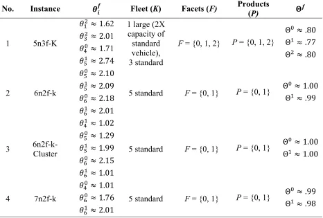
Table 1 describes the generated problem instances. The customer capacity utilization

ratio in (10) represents the ratio of the total demand of customer i divided by the capacity

available in a standard vehicle k, all in terms of facet f. When 1, more than one vehicle is

required to deliver the demand of customer i. If 1 2 then one large vehicle, if available,

could carry the total weight required by customer i (Because a large vehicle is assumed to have

twice the capacity of a standard one). Similarly, if 2 then not even a large vehicle could

singlehandedly supply the entire demand of customer i. In some cases, the demand of a certain

customer i may be such that it does not exceed the capacity of a vehicle in terms of one facet, but

subset thereof. Similarly, Θ in (11) is the total demand to total available capacity (System-wide)

ratio in terms of facet f. From here follows that if some Θ 1 then the instance is infeasible

because there is not enough total capacity across all vehicles to transport the required product by

all customers. The instances included in Table 1 describe some characteristics of the instances

included in this analysis. These instances were solved to optimality in an Intel Core i7 CPU with

8 GB of memory and running Windows 10. The VRPC was coded in OPL and ran on IBM Ilog

CPLEX with a branch and bound algorithm. Unless otherwise noted in table1, 1 ∀ .

Table 1 - Preliminary test instances for the VRPC

No. Instance Fleet (K) Facets (F) Products _(P)

1 5n3f-K

1.62 2.01 1.71 2.74

1 large (2X capacity of standard vehicle), 3 standard

F = {0, 1, 2} P = {0, 1, 2}

Θ .80

Θ .77

Θ .80

2 6n2f-k

2.10 2.09 2.18 2.01

5 standard F = {0, 1} P = {0, 1} Θ_Θ 1.00_.99

3

6n2f-k-Cluster

1.02 1.29 1.99 2.15 1.01

5 standard F = {0, 1} P = {0, 1} Θ 1.00

Θ 1.00

4 7n2f-k

1.01 1.76 2.01

5 standard F = {0, 1} P = {0, 1} Θ_Θ .99_.98

In addition to the capacity utilization ratios mentioned in Table 1, the following

parameters were used to define the problems. The three facets included in the problems were f =

capacity (homogeneous) or there is one larger vehicle (heterogeneous). Product magnitudes

were set such that each commodity p was significantly larger than the other two, in terms of one

facet f. Each customer was given a fixed set of coordinates and the cost matrix cij was obtained

based on Euclidean distances amongst each customer pair. In addition, the large vehicle was

given a cost factor of 1.5 that was used to account for any additional expenditures that a large

vehicle would incur when compared to the smaller vehicles. Thus ∙

depending on vehicle’s k cost factor.

Results of preliminary experiments

Table 2 includes the results of each optimal solution when solved using VRPSD (split

delivery without shipment consolidation) and in the third column, the objective function value

when the same instance is solved using the proposed model of VRPC (with shipment

consolidation). Finally, the last column shows the comparisons of the optimal solution value of

both models. As expected, the proposed model of VRPC performed better than the split-delivery

only model. A graphical comparison of both models follows.

Table 2 - Optimal solution values for the VRPC vs. VRPSD

Instance VRPSD VRPC Gap

5n3f-K 322.81 298.95 -7.39%

6n2f-k 232.54 229.17 -1.45%

6n2f-k-Cluster 319.11 306.60 -3.92%

7n2f-k 314.99 302.07 -4.10%

Figure 2 illustrates the optimal solution to 5n3f-K obtained through VRPSD. As

evidenced by the graph, all the vertices are visited by at least two vehicles. In addition, vehicle k2

is performing the longest route by visiting every node except 1. With 7.39% savings, Figure 3

shows the same instance solved with the proposed model VRPC. In this case, vehicle k2 is

consolidation that is taking place at customer 3 (k2 transfers 328 item of p1 to k3 so k3 alone can

fulfill the demand of customer 2). Moreover, in Figure 2 vehicle k1 must visit {5,4} alongside k2.

However, with VRPC this is no longer necessary as k1 makes a single-customer tour to 5

carrying p1 = 814 units to fulfill the demand of 5 (200) and to restock k2 from 1386 to 2000. This

enables k2 to visit 4 by itself, thus reducing total distance traveled.

Figure 2 5n3f-K with VRPSD Figure 3 5n3f-K with VRPC

Figure 4 depicts 6n2f-k’s optimal solution with VRPSD. In this case, both solutions are

surprisingly similar. The difference lies in Figure 5 in which consolidation takes place by

restocking p1 from 862 to 912 in k3 at customer 6’s location. This subtle change only results in

1.45% savings in distance traveled. However, this exemplifies how VRPC can produce savings

Figure 4 6n2f-k with VRPSD Figure 5 6n2f-k with VRPC

Instance 6n2f-k-Cluster is illustrated in Figure 6 with VRPSD and in Figure 7 with

VRPC. This heterogeneous-fleet, 2-facet, 6-customer problem is differentiated because nodes 2

and 6 are clustered at the right side of the coordinate plane, with customer 1 located somewhere

between the customer cluster and the depot. Figure 6 shows how without dynamic cross-docking,

vehicle k1 must travel across the four-vertex polygon comprised of {0, 5, 6, 1}. With VRPC,

Figure 7 changes the routing such that i) k1 is restocked at customer 6’s location as its load of p1

increases from 862 to 1086; and ii) k2 increases its cargo of p0 at node 4 such that it can visit

customer 1 and satisfy its product demand with no longer the need for a split delivery.

Figure 6 6n2f-k-Cluster with VRPSD Figure 7 6n2f-k-Cluster with VRPC

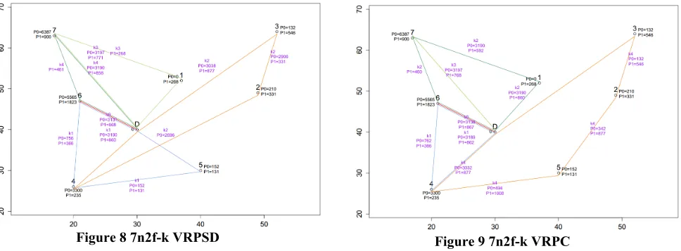
Finally, Figure 8 and Figure 9 show the sample instance 7n2f-k, which includes seven

maintained. After running the proposed model of VRPC (Figure 9) a consolidation point is

created at customer 4. Here, the cargo of vehicle k4 is increased from p1=877 to 1008. This

operation allows k4 to do the tour {0, 4, 5, 2, 3} in contrast to {0, 3, 2, 4} with the VRPSD

(Figure 8). By adding node 5 to k4’s route k1 no longer has to visit 5 and thus considerable

distance is saved (4.10%).

Figure 8 7n2f-k VRPSD _{Figure 9 7n2f-k VRPC}

The experiments herein mentioned briefly provide evidence as to the performance of the

proposed model for the VRPC. By adding possible shipment consolidation points, the convex

hull of feasible solutions includes more alternatives to solve the routing problem, while using

similar resources and offering the possibility for considerable savings. In some cases, such as

6n2f-k, there are only slight changes made to the routes. However, the power of VRPC resides in

the fact that even if a certain problem cannot benefit from consolidation, the optimal solution

will be at least as good as any obtained with a previously demonstrated model to have excellent

performance, such as VRPSD.

Computational experiments

To analyze the circumstances under which the proposed model for the VRPC performs

routing problem and it represents a multi-commodity, multi-dimension, heterogeneous fleet,

split-delivery routing problem, with mid-route shipment consolidation. Furthermore, the VRPC

includes facets, or various measures of each commodity from multiple dimensions (e.g. weight,

volume, value). Thus, there are no, to the best of the author’s knowledge, available instances to

use as a benchmark. For this reason, the instances used in this study were randomly generated, as

follows. First, the typology of the network may affect the viability of transferring commodities

across vehicles. Shipment consolidation may be particularly beneficial in cases where customers

are somewhat clustered, or in those in which few customers are scattered away, while most of the

customers are located somewhat close to one another. The variance of the arc length was

manipulated across high and low levels. Second, businesses with fleets of divergent capacities

can take advantage of larger vehicles, by using them as a mobile replenishment depot that can

reload smaller, cheaper to run, vehicles as they traverse the network. Two levels have been

defined based on this assumption: a homogeneous fleet wherein all vehicles have the same

capacity; and a heterogeneous kind in which the fleet has exactly one vehicle with twice the

capacity of the others. Third, studies have shown how patterns in customer demand can

dramatically affect the performance of some models. Under this assumption, each customer’s

demand variance of each product is altered across two levels. Finally, to assess the impact of the

size of the customer base, the number of nodes in the problem is changed. However, due to

computational limitations, only small cardinalities of the customer set (|N| = 5 through 10) were

solvable to optimality within reasonable amounts of processing time. Commodity magnitudes

were set such that each commodity ∈ 0,1 was larger than the other, in terms of one facet

∈ 0,1 . Thus, 2 and 2 . Finally, vehicle capacities , were

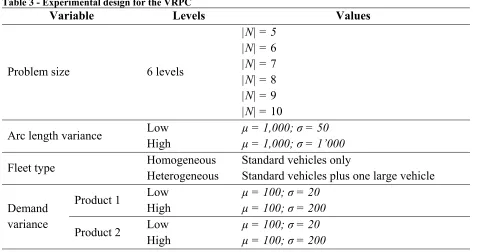
The full-factorial experimental design has a total of 96 combinations (6 x 2 x 2 x 2 x 2) of

the variables of interest. For each combination, 15 random problems were generated following

normally distributed random variables with the corresponding parameters from Table 3. This

translates to a total of 1’440 different problems. These problems were then solved with both the

proposed VRPC model and the VRPSD (split deliveries are allowed but commodities cannot be

consolidated across vehicles). This design raised the total number of problems to 2’880, out of

which 2’874 were solved (6 problems in one combination of the variables of interest triggered a

failsafe in the program code to prevent excessive solution times). Each problem was generated in

Java (JDK and JRE 1.8) and solved using IBM Ilog CPLEX version 12.6.3. The experiments

were conducted in a quad-core Intel Core i7 machine with 16 GB of memory running Windows

10. Some of the Java and CPLEX parameters were adjusted to maximize computational resource

utilization and keep the solution time within reasonable limits.

Table 3 - Experimental design for the VRPC

Variable Levels Values

Problem size 6 levels

|N| = 5 |N| = 6 |N| = 7 |N| = 8 |N| = 9 |N| = 10

Arc length variance Low

High

µ = 1,000; σ = 50 µ = 1,000; σ = 1’000

Fleet type Homogeneous Standard vehicles only

Heterogeneous Standard vehicles plus one large vehicle

Demand variance

Product 1 Low µ = 100; σ = 20

High µ = 100; σ = 200

Product 2 Low µ = 100; σ = 20

Results

The objective of computational testing is to evaluate the benefits obtained via the

proposed concept of shipment consolidation (VRPC) against a traditional model of vehicle

routing with split deliveries (VRPSD). Table 4 describes the different combinations of variables

of interest (cells), aggregated by problem size. That is, each cell represents the results obtained

Table 4 - Performance of the proposed VRPC against the VRPSD, aggregated by problem size

Experimental variables VRPSD VRPC

Cell _length) σ(arc σ(demand _P

1)

σ(demand

P2) Fleet

Time (Min)

Average SD

Time (Min)

Average SD

Average XD

Average Gap

1 50 200 200 0 3.89 5.19 0.91 5.20 2.31 -0.28%

2 50 200 200 1 1.81 4.58 2.08 4.07 2.12 -1.70%

3 50 200 20 0 1.91 4.48 0.79 4.78 1.52 -0.04%

4 50 200 20 1 1.40 3.92 0.95 3.58 1.26 -0.53%

5 50 20 200 0 2.32 4.56 1.41 4.59 1.23 -0.47%

6 50 20 200 1 0.43 3.88 0.35 3.71 1.41 -0.54%

7 50 20 20 0 2.82 3.87 2.13 3.92 0.62 0.22% 8 50 20 20 1 0.18 3.20 0.06 3.10 0.46 -0.44%

9 1000 200 200 0 9.09 5.01 5.75 4.94 1.53 -1.35%

10* 1000 200 200 1 6.77 4.29 0.88 4.10 1.53 -5.94%

11 1000 200 20 0 6.57 4.18 4.56 4.49 0.80 -1.11%

12* 1000 200 20 1 2.99 3.60 0.68 3.49 0.79 -3.50%

13 1000 20 200 0 4.70 4.18 2.27 4.37 1.03 -0.97%

14* 1000 20 200 1 2.69 3.30 0.57 3.36 1.03 -3.52%

15 1000 20 20 0 2.36 2.96 1.05 3.46 0.36 -0.58%

16 1000 20 20 1 0.19 2.30 0.04 2.18 0.21 -1.08%

Total 3.13 3.97 1.53 3.96 1.14 -1.36%

Notes: SD and XD is the number of nodes in which a split delivery and product consolidation takes place, respectively. A more negative gap implies better performance of the VRPC vs. the VRPSD

Fleet is equal to one when the generated problem had a heterogeneous fleet, homogeneous otherwise * top three-performing combinations (cells) of the full-factorial experimental design

Savings potential

Results on Table 4 highlight the savings potential that shipment consolidation can entail.

The Gap column is the average percent change observed when using the VRPC vs. using the

VRPSD (A more negative gap value indicates larger savings due to the VRPC). Aggregating the

entire results, across all 2’880 problems solved, showed an average improvement of the objective

value of 1.5 percent due to the VRPC. This finding suggests that, on average, it is more

beneficial to implement shipment consolidation and improve the fleet’s utilization. The

best-performing cells in the experimental design were: 10, 14, and 2. These combinations

revealed an average improvement in the objective function value (lower value) of 6, 3.5, and 3.5

percent, respectively over 90 different problems solved in each of them. These cells appear to

have higher variances in common. They all have highly varying arc lengths and, the demands of

either product 1 or 2, or both. Furthermore, all these instances belong to cells with heterogeneous

fleets. This suggests that the more scattered the customers and the more variant their demands

are, coupled with a heterogeneous fleet, the higher the savings potential of the VRPC and its

mid-route shipment consolidation capability.

Split delivery and consolidation behavior

The average number of consolidation sites (Avg XD or, the number of customer sites

where payload consolidation occurs) is slightly greater than one (1.14) across all problems. This

signals that transferring payload from one vehicle to another, in at least one opportunity, during

all the routes in the fleet, can offer important savings. While the VRPC does rely on transferring

payload across vehicles at a customer location, using such model does not appear to change the

number of times a customer is visited on average. This is supported by the fact that the average

(Paired t-test t = -0.88376, df = 959, p-value = 0.1885). While some of those deliveries may

involve shipment consolidation, the average number of split deliveries remains statistically

comparable. See Figure 10 below.

Figure 10 - Number of split deliveries (SD) in the VRPC vs. the VRPSD

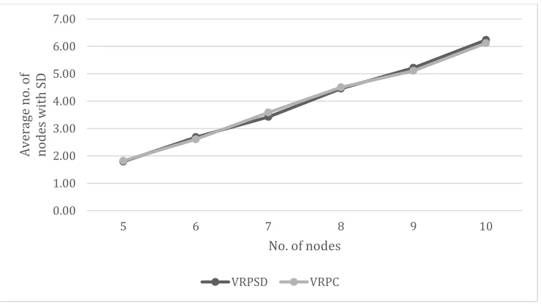
Consolidation, however, seemed to be positively correlated to the problem size. See

Figure 11, next. As shown by the results grouped by problem size, the number of customers

wherein payload transfer across vehicles takes places seems to increase as a factor of the number

of nodes in the network. This outlines the possibly greater benefits of implementing the proposed

VRPC model on larger networks of customers. 0.00

1.00 2.00 3.00 4.00 5.00 6.00 7.00

5 6 7 8 9 10

Avera

ge no. of

nodes

with

SD

No. of nodes

Figure 11 - Number of nodes with mid-route shipment consolidation (XD)

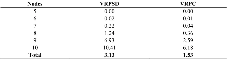
Computational time

Table 5 supports the expected time complexity of the problems. The computational times

required to reach optimal solutions increases alongside the number of nodes in the network. This

prevented further analyses using larger networks in which potentially better savings could be

obtained. A time limit of 30 minutes was set on algorithm runtime, at which point its execution

was terminated. If no optimal solution was reached, then a new problem was generated, and the

algorithms were restarted.

Table 5 - Average computation time per model

Nodes VRPSD VRPC

5 0.00 0.00

6 0.02 0.01

7 0.22 0.04

8 1.24 0.36

9 6.93 2.59

10 10.41 6.18

Total 3.13 1.53

Discussion

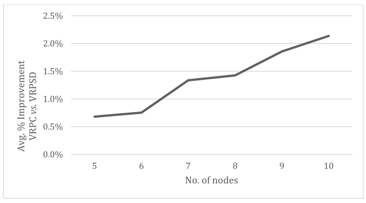
Results from the numerical experiments support expected benefits accrued due to the

VRPC. Reduced problem sizes attained nearly four percent savings in objective function value 0.00

0.20 0.40 0.60 0.80 1.00 1.20

5 6 7 8 9 10

Avera

ge no. of

nodes

with

XD